¶ Optimizing a Process
Optimization is finding the best solution or the most efficient way to achieve a specific goal, given certain constraints and conditions.
It is required to make the best use of available resources to minimize costs while maximizing profits. It provides a systematic approach to decision-making by identifying the best possible options for a goal.Today, most critical process industries are governed by control systems to automate how the process must react to changes. This is achieved through implementation of control loops.
However, the efficiency of a plant or a process is still driven by hourly/daily decisions made by operators on critical inputs based on which the loops will respond. Any sub-optimal decisions on these decisions can lead to losses which manifest as increased energy spend, poor quality of a product, incomplete processing, safety hazard etc.
For example, in an industrial asset combustion process, providing lesser air than required can lead to a reducing environment or safety hazard. Similarly, in a water treatment plant, performing lesser dosing than required can lead to poor quality of water.
Process optimization helps plant operators make the best decision to achieve a goal (like maximizing efficiency, minimizing input costs) within a constraint (like parameters must be within certain limits).
Optimization tool helps the plants to operate at best possible configuration during flexible operations, thereby reducing Heat Rate of the unit and cost of fuel.
The tool supports active combustion monitoring and reduced Auxiliary consumption by performing detailed specific power analysis.
¶ AI for Process Optimization
Traditionally, process optimization is taken up as a periodic exercise (monthly, annual) of manual data study using quantitative methods to identify strategy changes for process decision making. But this doesn’t help in a dynamic plant with frequent changes (like input quality, demand changes, etc) where decisions need to be made in a timely manner (more real-time) to avoid accumulation of losses. These methods are also insufficient in very complex processes with numerous interactions between various assets where manual studies are unable to capture all underlying dynamics.
This is where use of Artificial Intelligence helps plants push the boundaries to constantly make the best decisions in real-time to achieve the desired plant objectives. A real-time optimization system also helps a plant make consistent decisions irrespective of the operator or his/her experience thereby bringing about more stability in the plant.
In the current discussion, the optimization of combustion process, and environmental sustainability of combustion processes within Thermal industrial assets by addressing the factors impeding the efficient functioning of the equipment, are considered.
You get the five-minute forecast of the process in a graphical manner continuously for a selected tag (sensor). This helps plant engineers in monitoring the resources involved in the process. In the current example it is air and coal. Following the recommendations, you can ascertain the optimum levels by controlling the flow of resources through the Controllable option..
Inefficient combustion can lead to excessive energy consumption, increased emissions of pollutants, thereby raising the operational costs.
By improving the efficiency of the process, the auxiliary power consumption by the equipment can be minimized.
Models are created, trained and tested so as to get the best recommendations from the Recommendation engine.
¶ Pulse Process Optimization Engine
The optimization engine in Pulse was designed to learn from the historic context of complex processes and provide operators with real-time interventions in the form of setpoint recommendations (of controllable parameters) any time the process is deviating from the stated objectives.
Consider a Power Generation plant for example:
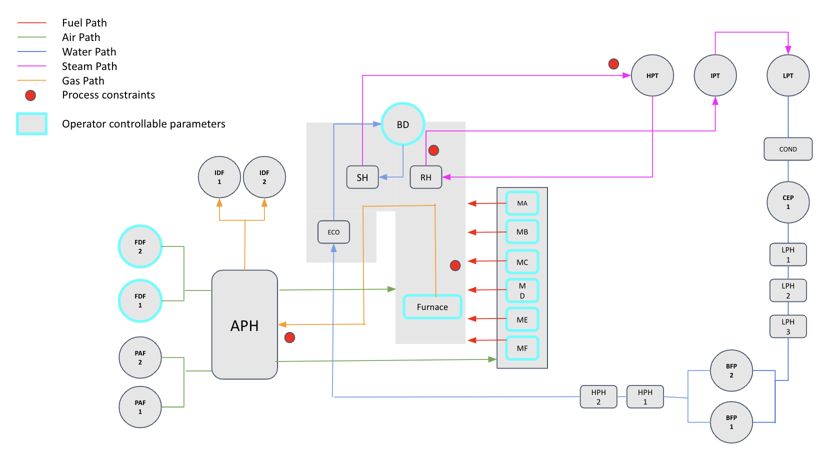
Figure 1. Schematic of a power plant
This is one of the more complex industries where there is an interaction between various media like Fuel (solid/liquid), Air (for combustion), Water (to convert to steam), Steam (to convert to rotational energy) and Flue Gas (to exchange heat) covered by 1000+ parameters. The overall plant efficiency (or heat rate) is dependent on use of the least amount of energy to maximize power generation.
In the above process:
Objective: Minimize the energy (fuel) input per unit of power generated
Constraints: The following are some of the constraints.
-
Excess O2 in flue gas
-
Flue gas exit temperature
-
Main steam temperature and pressure deviations
-
Reheat temperature and pressure deviations
-
Reheat spray flow consumption
-
Mill outlet temperature
-
Tube metal temperature
¶ Controllables:
-
Fuel input: Decision on fuel loading across all mills
-
Air input: Volume of air for combustion, FD Fan blade pitch or damper position
-
Sootblowing operations
¶ Configuring Pulse to achieve the optimization objectives
The Pulse optimization engine is designed as a zero-code interface to configure any plant process, define the interactions between the various assets of the plant and create a network of models that unearth the underlying process dynamics/relationships.
Some of the steps that goes into this are:
- Define the plant and process parameters
Setup the optimization engine with all the relevant parameters organized into logical groups (like Asset → Sub-system) and clear identification of which parameters are controllable by the operator and constraints on other key parameters.
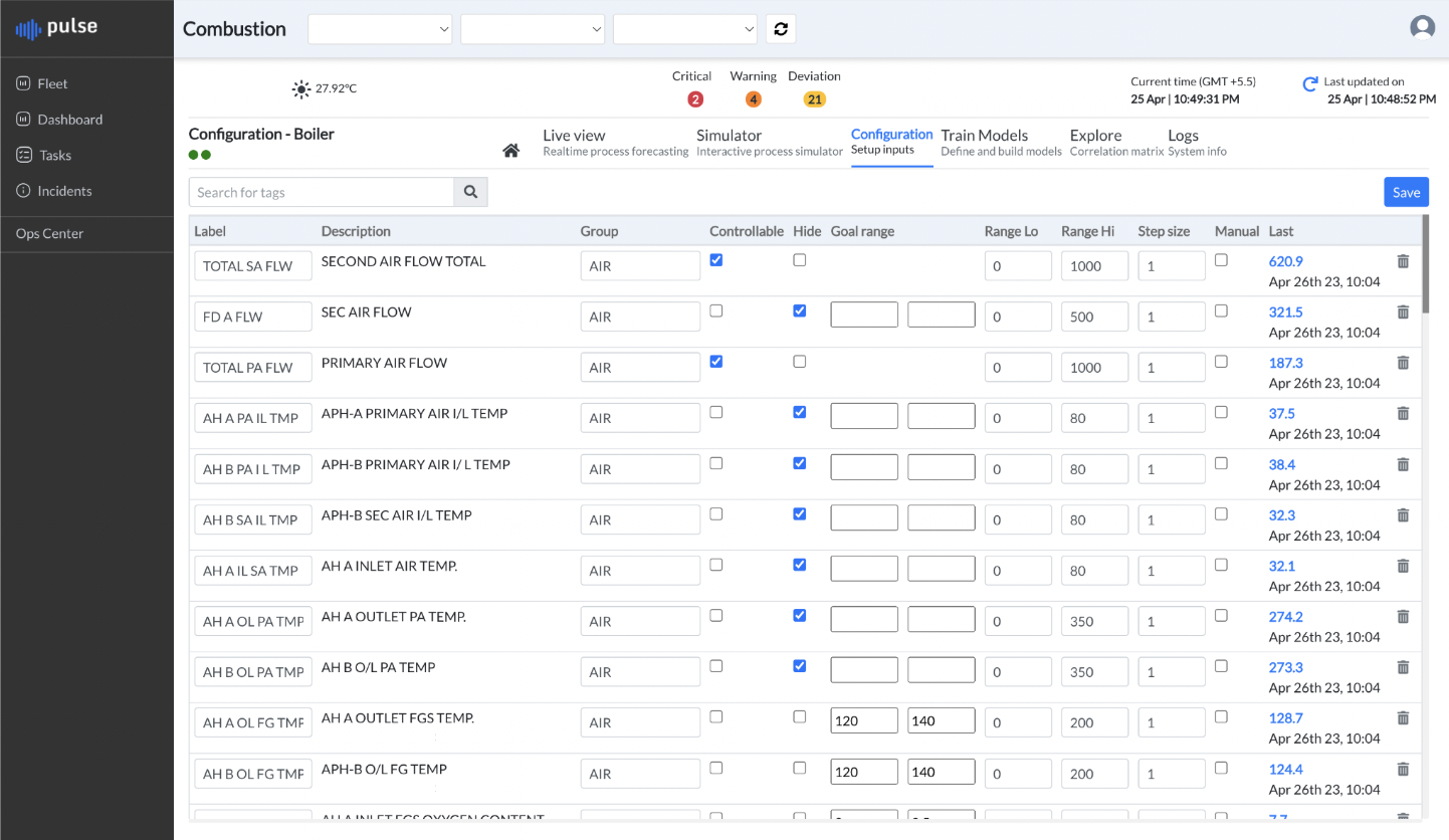
Figure 2. Combustion optimisation page
- Develop Models
Component/Asset level multi-variate models are built to understand the component’s response to changes in its inputs. Typically a series of such models are built for all the major components in the plant/process using neural networks.
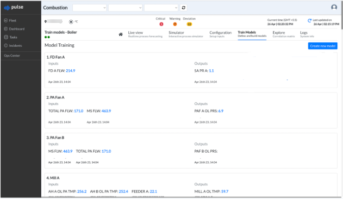
Figure 3. Train models tab
- Recommend or Simulate
The output of the optimization can be consumed in one of the following ways:
a. Notification of recommendation: Whenever the engine identifies that the process is moving away from its goals/objectives, it automatically scans through the entire series of models to identify possible changes to the controllable parameters that could help achieve plant goals while also checking if such changes meet the defined constraints.
The output is in the form of a workflow notification which clearly identifies the setpoint recommendations and the expected change to the plant objective parameter due the recommended change.
The engine also tracks operator actions (changes to the recommended setpoint parameter) to create an effective way of continuous learning for the optimization engine.
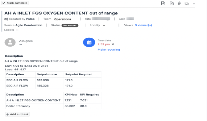
Figure 4. Optimisation task
b. Simulation Engine: This tool provides an on-demand way for operators to try out changes to the process to observe the impact on the objectives and constraints.
This could be a powerful tool for companies to train their operators and experiment with processes without actually making changes to the plant.
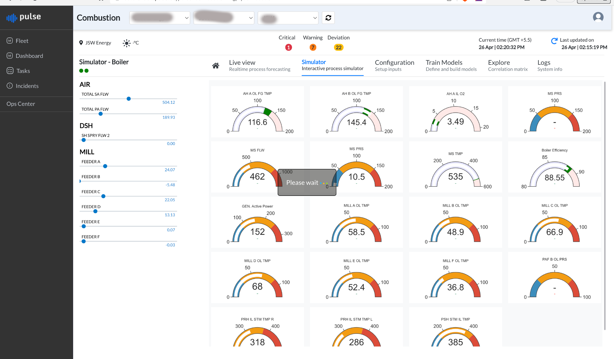
Figure 5. Simulator tab
The salient features of Optimization include:
-
Real time process forecasting
-
Simulation
-
Personalized process recommendations
-
Goal Setting
-
Enabling/Disabling Transient State of Systems
-
Enabling Number of Recommendations
-
Enabling Process Excursion Time Window
-
Customizing Criteria
-
Choosing Controllable Parameters
-
Setting Low/Hi Ranges
-
Building a Model
-
Creating a Model
-
Viewing Model Data
-
Training & Testing the AI model
¶ Viewing Simulation of a Process in Real Time
To view Simulation of a Process in real time:
- Click the Simulator tab
A simulation of the real time processes that are currently being carried out under that optimization appear
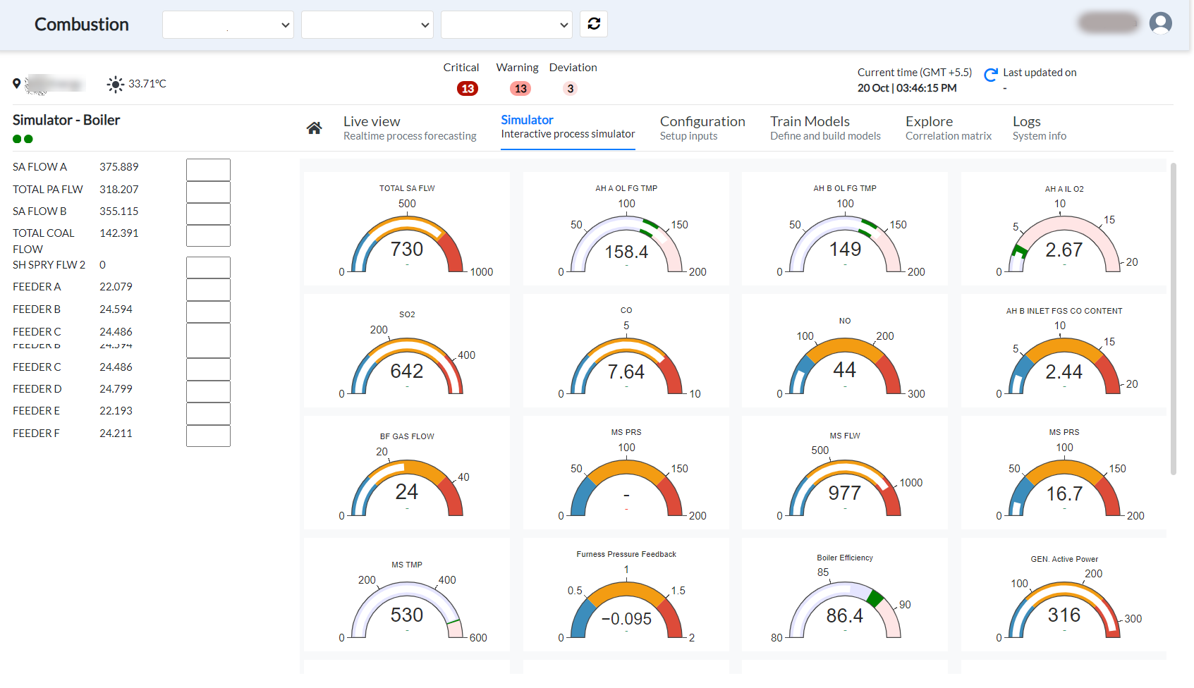
Figure 6. Simulator tab
When you change some controllable parameter values such as air flow or coal flow, the effect on the dependent parameter values show up indicating the +/- change under each parameter.For example,
-
Change the SA (L) value to 639.2.
-
Click Go.
The simulator starts running. All the output tags of the associated models reflect the change as increase or decrease in the current values that is shown in the dials.
The Simulator tab has the Refresh functionality.
- Click the tab,
Each time the values turn to 0 and are refreshed to new values at that point in time based on the process stage and equipment status.
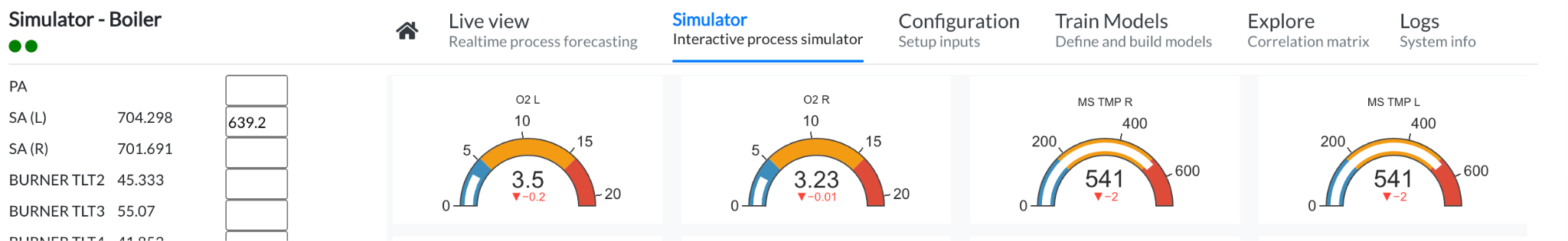
Figure 7. Values in simulator
¶ Configuring Tags
Do the following to configure tags.
- Click Configuration,
This page appears with the following fields.
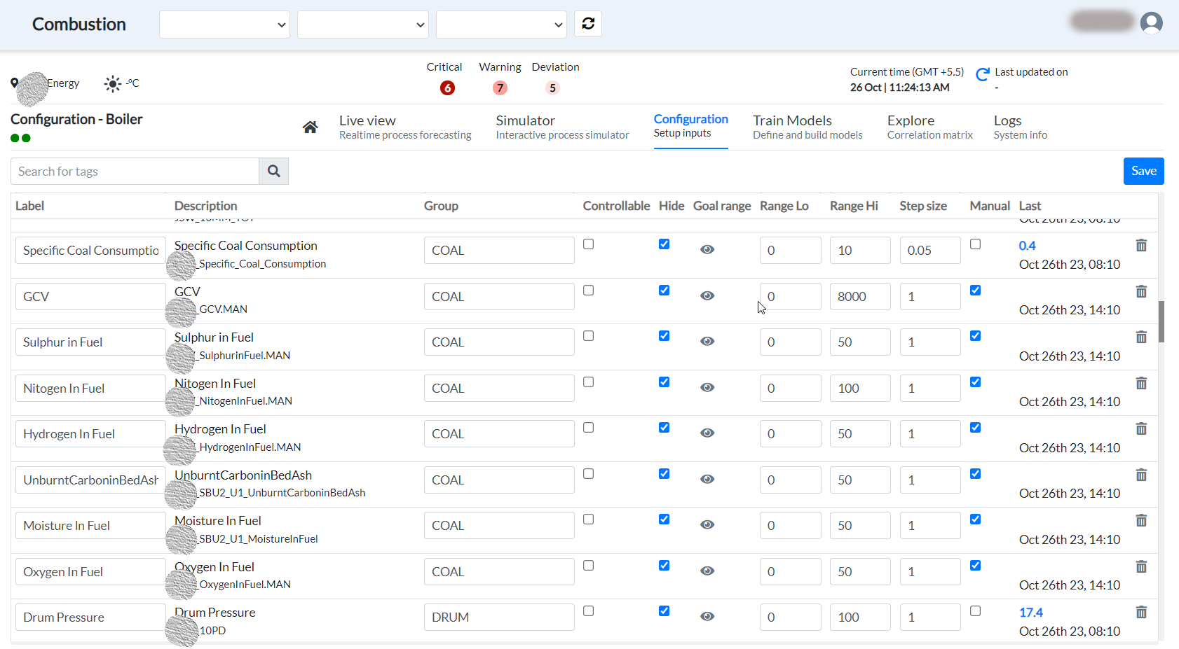
Figure 8. Configure tags tab
- Enter the tag description or its dataTagId. Then Click the search icon. The list of available tags appears.
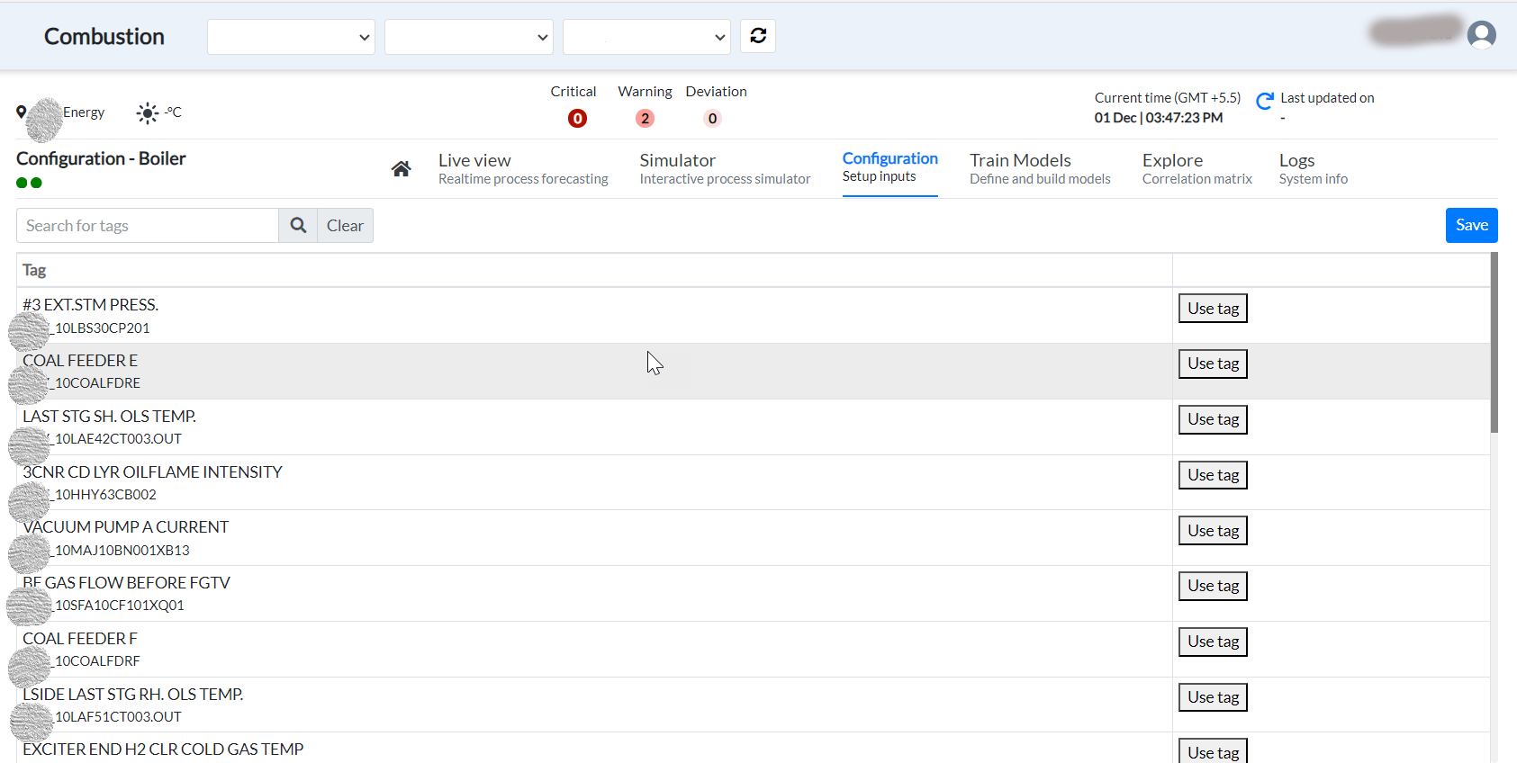
Figure 9. List of available tags
-
Click Use tag to use the tag.
-
Click Clear to go back to the Configuration main page.
i. Label - Edit the label of a tag if the description is not suitable.
ii. Group - Enter a system name such as COAL, AIR, ECO, APH, and so on corresponding to a tag to group the tags into that system category to view in an organized way in the Live view page.
iii. Controllable -. Select the checkbox if you want the tag to be editable and clear the corresponding checkbox to make the parameter view-only.
iv. Hide - Use this option to control what parameters to hide on the simulator page to reduce the clutter. By default the checkbox is clear, hence the parameter appears on the simulator page.
v.Goal Range - Use this option to set up a tag for initializing recommendations
¶ Enabling and Disabling Parameters under Configuration.
- Click the Eye icon, this page appears.
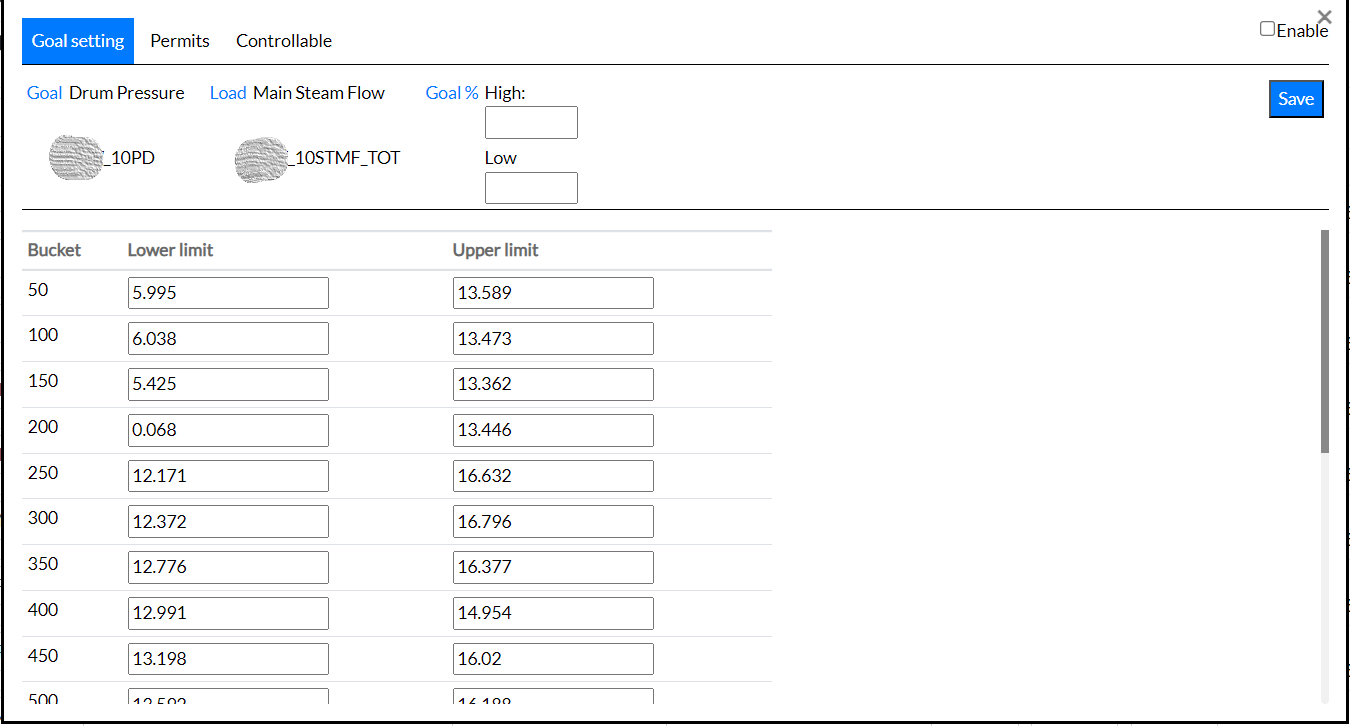
Figure 10. Goal setting tab
-
Select the Enable checkbox on the top right corner of the page.
-
Click Save after entering or selecting the values in the fields under the three tabs.
¶ Setting the Goal
To set a goal:
-
Select a quartile within each load bucket that the recommendation engine considers
-
Select or enter Goal% High.
-
Select or enter Goal% Low.
-
Click Reset ranges, to enter new values for bucket load ranges.
-
Click Save after you change or enter the values.
Note: The default quartile range is q20 to q80 of the goal tag’s benchmark Load. You can modify any of the values individually for any of the buckets.
Use the Permits tab to control how recommendations are run.
You can perform these activities in the Permits tab.
Click Permits.
The following page appears.
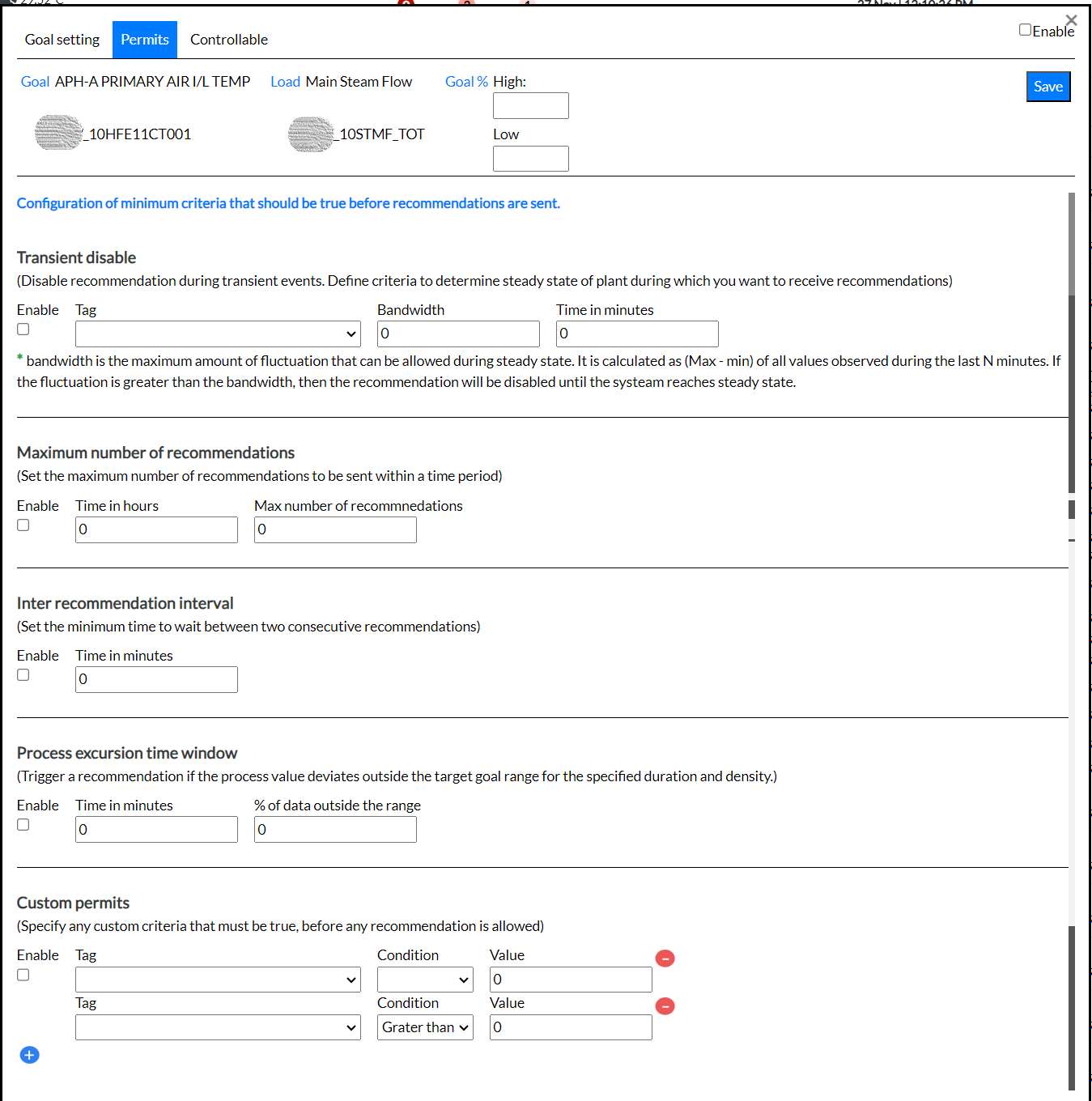
Figure 11. Permits tab
¶ Enabling/Disabling Transient State of Systems
To enable or disable the transient state of a system:
- Select the Enable checkbox in the Permits tab
The recommendation engine identifies if the system is in transient mode, Recommendations are avoided unless you select Enable.
- Select a proper Load tag from the Tag drop-down list. Set a bandwidth, under which only the recommendations are generated.
¶ Enabling Number of Recommendations
To enable Maximum number of recommendations:
-
Select the Enable checkbox.
-
Enter or select the time (in hours).
-
Enter or select the maximum number of recommendations/tasks.
¶ Enabling wait time Between Recommendations
To set waiting time for between recommendation:
-
Select the Enable checkbox.
-
Enter or select the wait time.
¶ Enabling Process Excursion Time Window
To set time window to trigger recommendation if process deviates the set time and density:
-
Select the Enable checkbox.
-
Enter or select the time (in minutes).
-
Enter or select the data density (percentage outside the range).
¶ Customizing Criteria
To customize criteria for triggering recommendation:
-
Select the Enable checkbox.
-
Select the tag from the drop-down list.
-
Select a condition - Greater than or Less than.
-
Enter or select a value.
¶ Choosing Controllable Parameters
Click Controllable.
The following page appears.
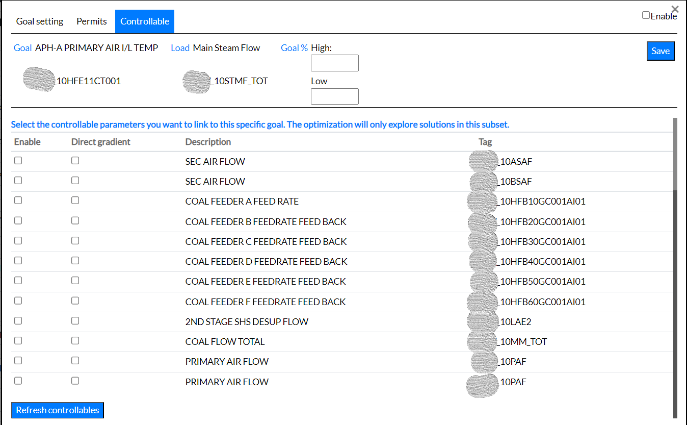
Figure 12. Controllable tab
To choose the controllable parameters:
-
Select the Enable checkbox.
-
Select the Direct gradient checkbox.
-
Click Refresh controllables to clear the checkbox selection.
- Click Enable at the right top of the dialog box after completing all the three tabs - Goal Setting, Permits, and Controllable.
¶ Setting Low/Hi Ranges
To set low and high ranges:
Enter or select values from Range Lo and Range Hi spin boxes.
¶ Setting Step Size
To set the step size:
- Enter or select a value
¶ Using Values from Data Entry page
- Select the Manual checkbox to treat the tag as Manual that comes from the daily Data Entry page, and the same value is used for that day to train the model. For example, GCV and Coal Moisture
¶ Saving the changes
- Click Save after completing all the fields in the .Configuration tab.
¶ Building a Model
To build a model:
Each model represents a specific equipment or process, whereas in the case of an output tag, all the relevant and impactful input tags are provided.
Multiple output and input tags can exist simultaneously.
Rules:
● A tag can be input to any number of models.
● For an output tag, only one model can exist.
¶ Creating Model
To create model:
- Click the Train Models tab.
The Model Training page appears.
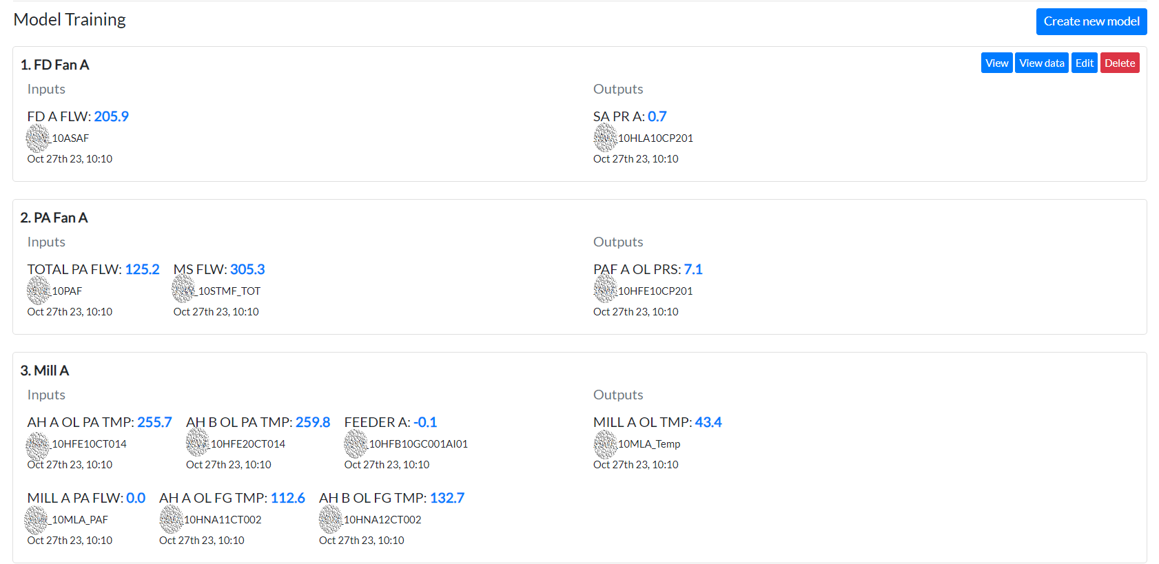
Figure 106. Model training page
- Click Create New Model in the Model Training page.
New options appear on the Model Training page as shown.
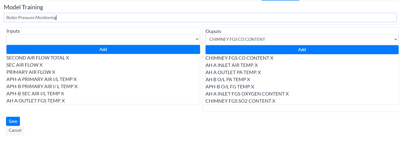
Figure 13. Input and output tags
Use these options to create a new model for the equipment.
-
Enter a name for the model you are creating. We have entered the name Boiler Pressure Monitoring in this example.
-
Select an Input from the Inputs drop-down list and click Add to add an input parameter.
-
Select an Output from the Outputs drop-down list and click Add to add an output parameter.
-
After adding the input and output parameters, click Save to update the data.
The newly created model appears on the Train Model page under the list of models, where the options to View, View data, Edit and Delete a model are shown.
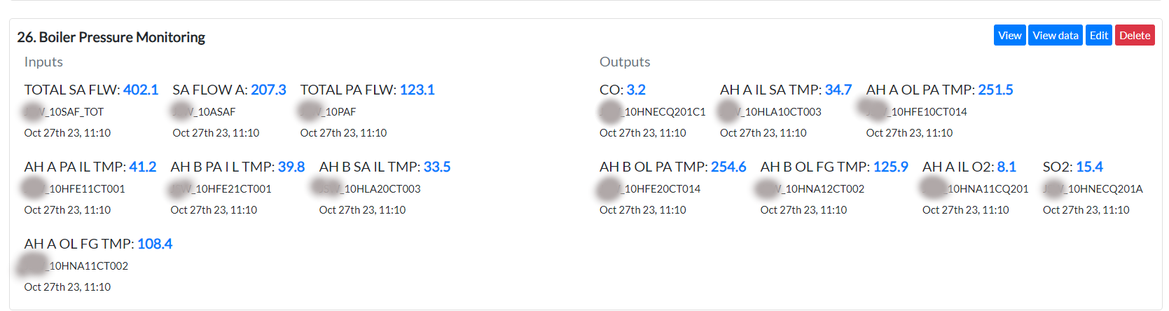
Figure 14. Model
¶ Viewing Model Data
To view Model Data for a version:
- Click View to view the data of the model for a particular version.
The page shown here appears.
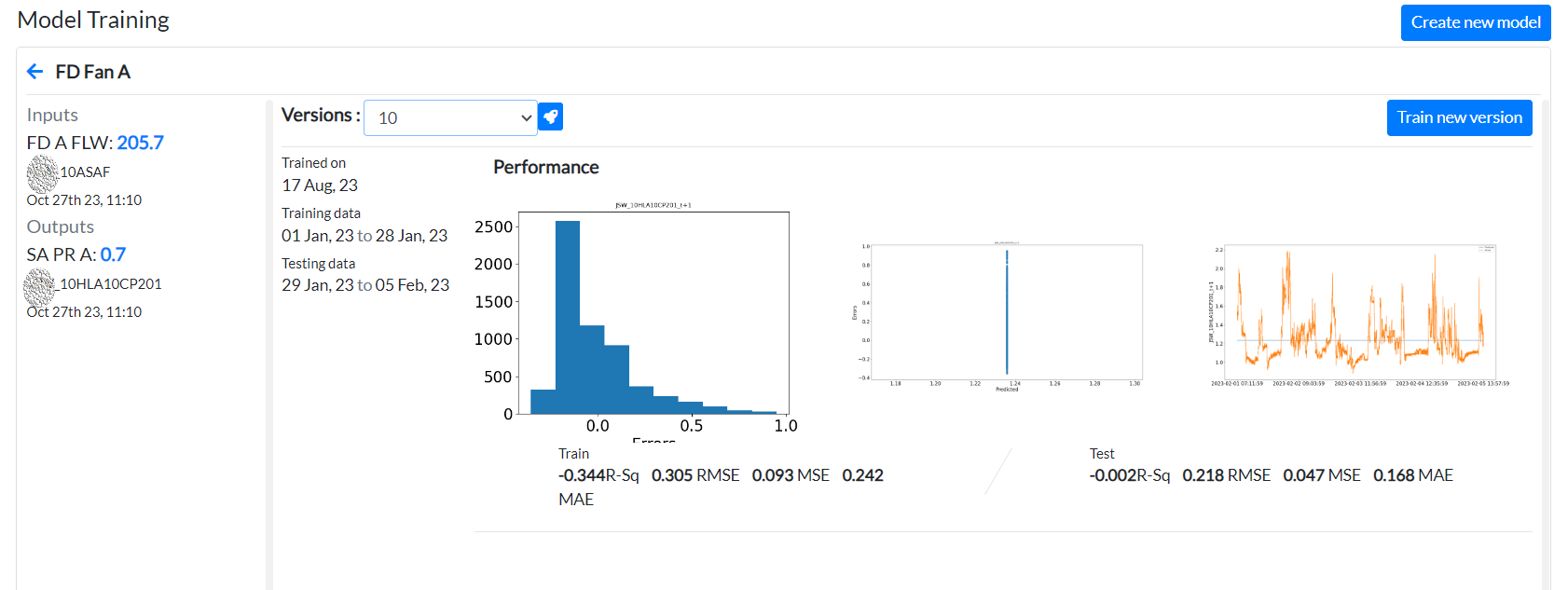
Figure 15. Model performance tab
- Select a version from the Versions drop-down list to view the data for that version of the model.
The page has these details:
● Versions of models that are trained.
● Deploy/Retire the selected model.
(Click the Deploy(blue) and Retire(red) icons to complete the actions.)
When you select a version the following graphs appear:
-
Performance graphs of “Test data”:
-
Error histogram
They show Predicted versus error and Actual versus predicted values
¶ Editing Model Data
To edit a model data:
- Click Edit in the row.
The Inputs and Outputs drop-down menus appear.

Figure 16. Input and output dropdown
-
Select an Input from the Inputs drop-down list and click Add to add an input parameter.
-
Select an Output from the Outputs drop-down list and click Add to add an output parameter.
-
Click Save to save the changes.
¶ Training & Testing a Model
To train and test a model:
- Click Train new version to train the model on another version.
This page appears.
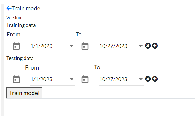
Figure 17. Dialog box to choose train and test data
-
Click the calendar icons under Training data and Testing data to change the starting and ending dates.
-
Click the + icon to add a fresh row of date range.
-
Click the X icon to delete a row of date range.
-
Click Train model to add the new version of the model.
¶ Exploring Equipment Parameters
To explore the equipment parameters:
- Click the Explore tab.
This page appears with the parameters in a tabular matrix format along with the scatter plotting of the correlation.
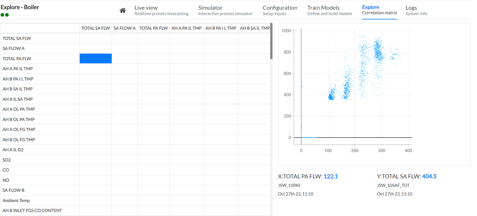
Figure 18. Explore tab
- Click a cell in the matrix, the scatter plot of the corresponding values appears alongside.
¶ Viewing Model Training Logs
- Click the Logs tab,
The logs of models being trained are displayed.
After the model training starts, it shows training has been started,
After training is completed, it shows model training has been completed.