¶ Introduction
The Characteristic Curve is a visualization feature available within the Dashboard section of Pulse, designed to provide a clear comparison between design performance and actual operating performance of industrial equipment such as pumps and compressors.
At its core, this feature transforms the static performance curves provided by the client into a dynamic, real-time analytical tool. It enables users to visually assess whether the equipment is operating within its expected performance range and identify any deviations that may indicate inefficiencies or potential issues.
¶ Conceptual Understanding of the Characteristic Curve
From the client side, the starting point is typically a datasheet performance graph. This graph represents how the equipment is expected to behave under different operating conditions.
For example, in the provided datasheet:
- The X-axis represents Capacity (Flow in m³/hr)
- The Y-axis represents parameters such as Efficiency, Head, or Power
Below is an example of performance curve shared by the client according to which user wants to check the values
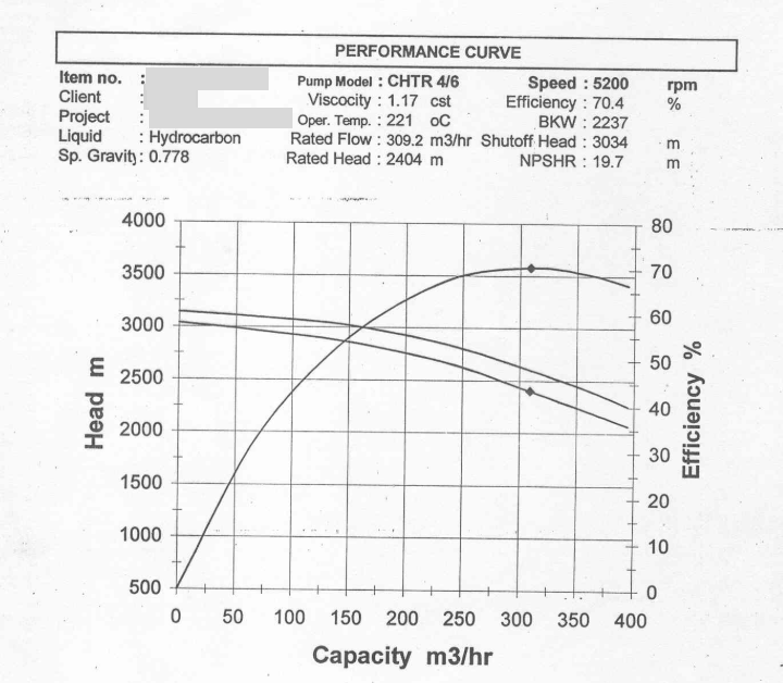
Figure 1. Conceptual Understanding of the Characteristic Curve
In Pulse, this entire concept is translated into a simple idea:
“What should happen” (design curve) is continuously compared with “what is happening” (real-time data).
¶ How the Curve is Created in Pulse
The creation of the characteristic curve is not manual plotting but a structured transformation process.
Initially, the graph provided by the client is digitized. Multiple points along the curve are identified, and their corresponding X (Flow) and Y (Efficiency/Head/Power) values are extracted.
These extracted points are then used to generate a mathematical representation of the curve. Instead of plotting discrete points, Pulse fits a smooth curve using regression.
y= a_0 + a_1 x + a_2 x^2 + a_3 x^3 y=a0+a1x+a2x2+a3x3
y = intercept + x * x + x2 * x^2 + x3 * x^3
This equation allows the system to:
- Recreate the curve accurately
- Generate values for any intermediate point
- Maintain smoothness and continuity
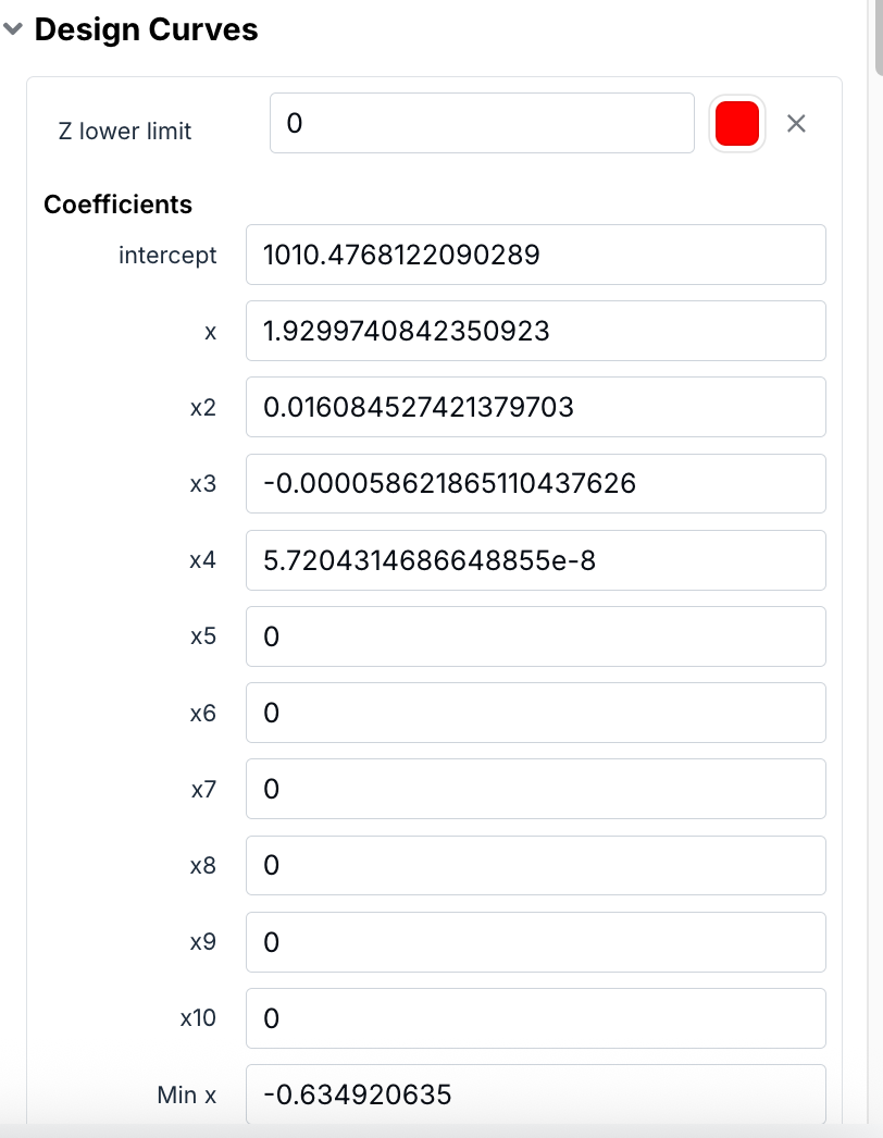
Figure 2. How the Curve is Created in Pulse
While generating the characteristic curve, the system uses a polynomial equation derived from the extracted data points. The accuracy of this curve depends on the degree of the polynomial used.
A lower-degree polynomial (for example, linear) results in a simpler curve, whereas higher-degree polynomials allow the system to better match more complex shapes from the client’s datasheet.
In practical implementation:
- A simpler curve may use fewer coefficients
- A more complex curve requires higher-degree terms
The degree is selected iteratively to ensure that:
The generated curve closely resembles the original client-provided performance curve.
This approach ensures both visual accuracy and mathematical consistency of the curve within the system.
¶ Tag Value Range Constraint
When configuring the characteristic curve, it is important to ensure that the selected tags produce values within the defined X-axis range.
For example:
- If the X-axis (Flow) range is defined from 0 to ~390
- Then any tag mapped to the graph must produce values within this range
If tag values fall outside this range:
- The data points may not be plotted correctly
- The curve visualization may not behave as expected
Therefore, while assigning tags:
It is essential to ensure that the selected data aligns with the configured axis limits.
¶ Mandatory Tag Configuration Requirement
The system requires a minimum number of tags to successfully create and save a characteristic curve.
- At least three tags must be configured
- Each tag must be assigned to an axis (X, Y, or Z)
Even in cases where the Z-axis is not functionally required (such as pump-based curves), a third tag is still needed to satisfy the system configuration requirement.
This ensures consistency in how characteristic curves are structured within the platform.
Figure below shows a curve recreated with this above steps
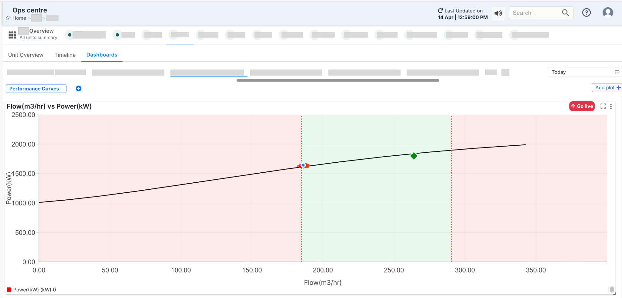
Figure 3. Mandatory Tag Configuration Requirement
¶ Axis Configuration and Their Meaning
The axis configuration depends on the type of equipment being monitored.
For pumps, the system works with a straightforward two-axis configuration:
- X-axis: Flow (m³/hr)
- Y-axis: Parameter (Efficiency, Head, or Power)
Since pump performance does not vary across multiple operating layers like speed curves, a third axis is not required.
In contrast, for compressors, an additional dimension is often needed. In such cases:
- The Z-axis represents operating conditions such as speed (RPM)
- Multiple curves may exist for different speeds
This allows the system to represent more complex performance behavior where the same flow may result in different outputs depending on operating conditions.
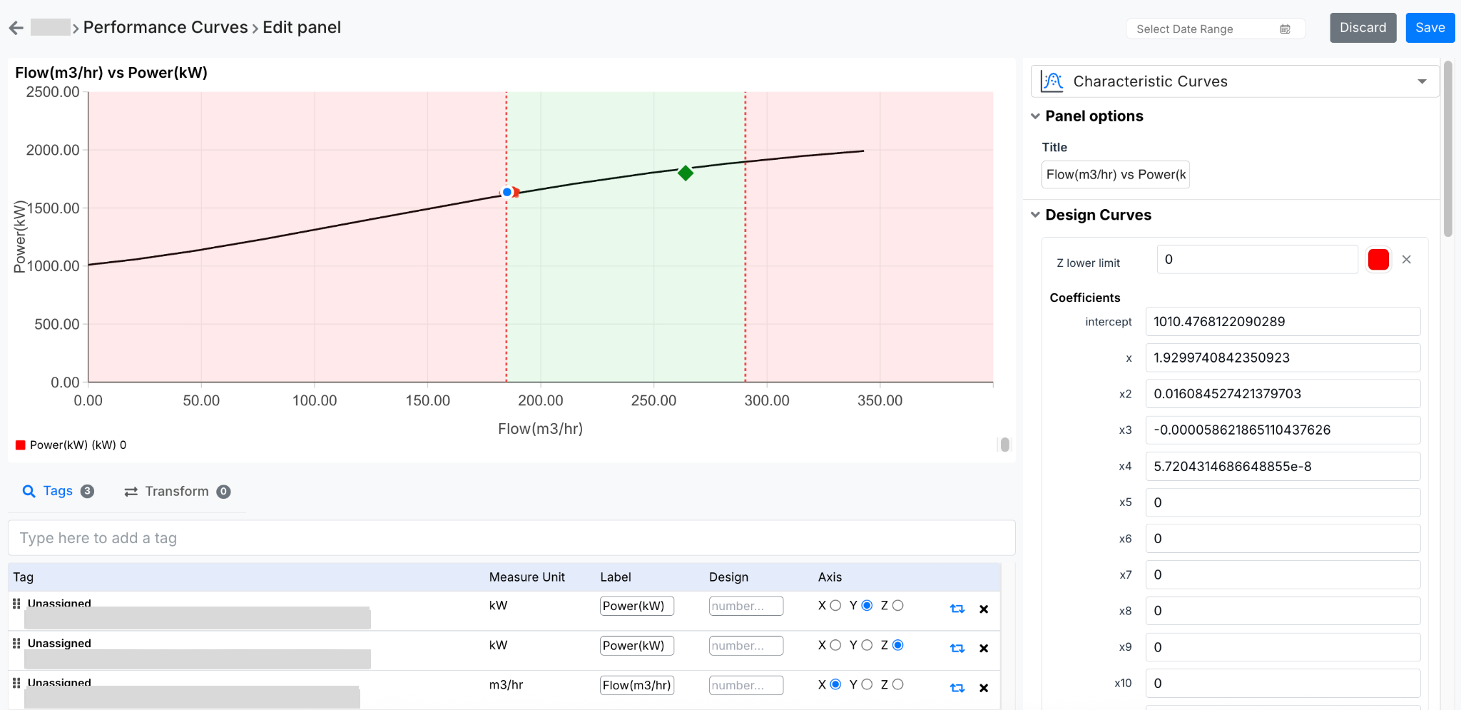
Figure 4. Axis Configuration and Their Meaning
Once the curve is established, the next step is mapping real-time data onto it.
Each axis is linked to specific tags:
- Flow is typically a raw sensor value, converted into standard units (m³/hr)
- Efficiency, Head, or Power are either measured or calculated values
As data flows into the system, it is plotted dynamically on the graph. This creates a continuous comparison between:
- The design curve (black line)
- The actual operating point (blue marker)
When the user hovers over the graph, detailed values are displayed, including:
- Actual vs design values
- Timestamp
- Marker information (BEP, Rated point)
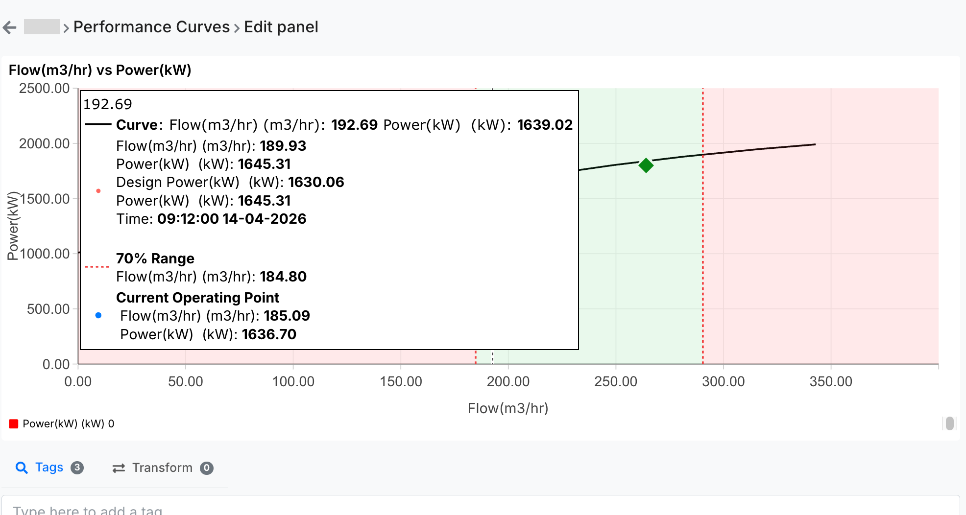
Figure 5. Real-Time Data Mapping
Markers are one of the most important additions to the characteristic curve feature, as they provide clear reference points defined by the client.
These are not system-generated assumptions—they are based on actual datasheet values provided by the client.
¶ Types of Markers
Typically, two primary markers are used:
- Rated Point
Represents the standard operating condition of the equipment - Best Efficiency Point (BEP)
Represents the point at which the equipment operates at maximum efficiency
In many cases, both values are the same unless explicitly specified otherwise in the datasheet.
Nature of BEP and Rated Values
The BEP (Best Efficiency Point) and Rated values are derived from the equipment datasheet and represent design parameters.
These values:
- Are not dynamically calculated
- Remain constant unless manually updated
Since they represent design characteristics, any changes would require manual reconfiguration in the system.
Each marker is defined using:
- X value (Flow)
- Y value (Efficiency / parameter)
- Label, color, and size
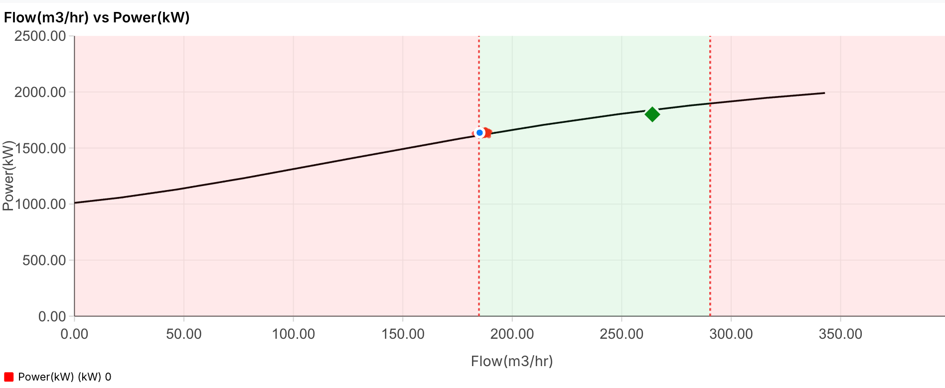
Figure 6. Types of Markers
Note: The color used for markers (such as green in the current configuration) is not fixed or predefined. It is selected purely for visual distinction and better readability of the graph. Marker colors can be customized as required, and there is no dependency or logic tied to a specific color.
¶ BEP-Based Operating Range
One of the key client requirements is the visualization of the acceptable operating range around the BEP (Best Efficiency Point).
This is implemented by calculating a range based on the BEP flow value:
- 70% of BEP flow
- 110% of BEP flow
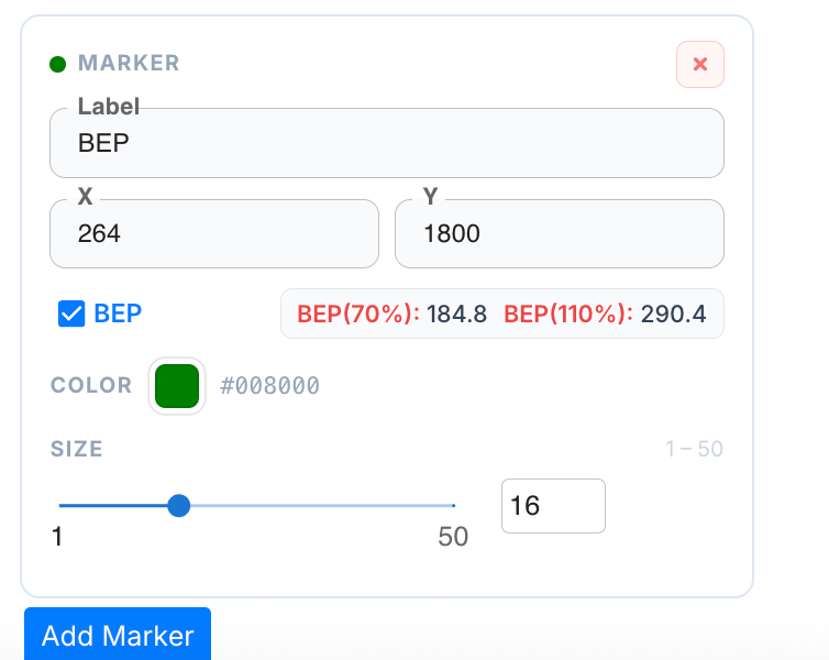
Figure 7. BEP-Based Operating Range
- BEP Flow = 239 m³/hr
- 70% = 184.02 m³/hr
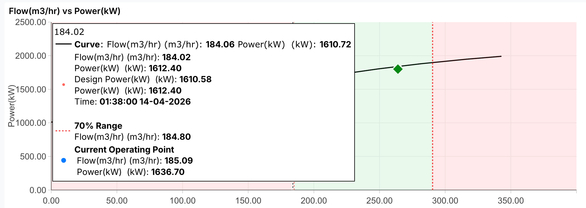
Figure 8. 70% = 184.02 m³/hr
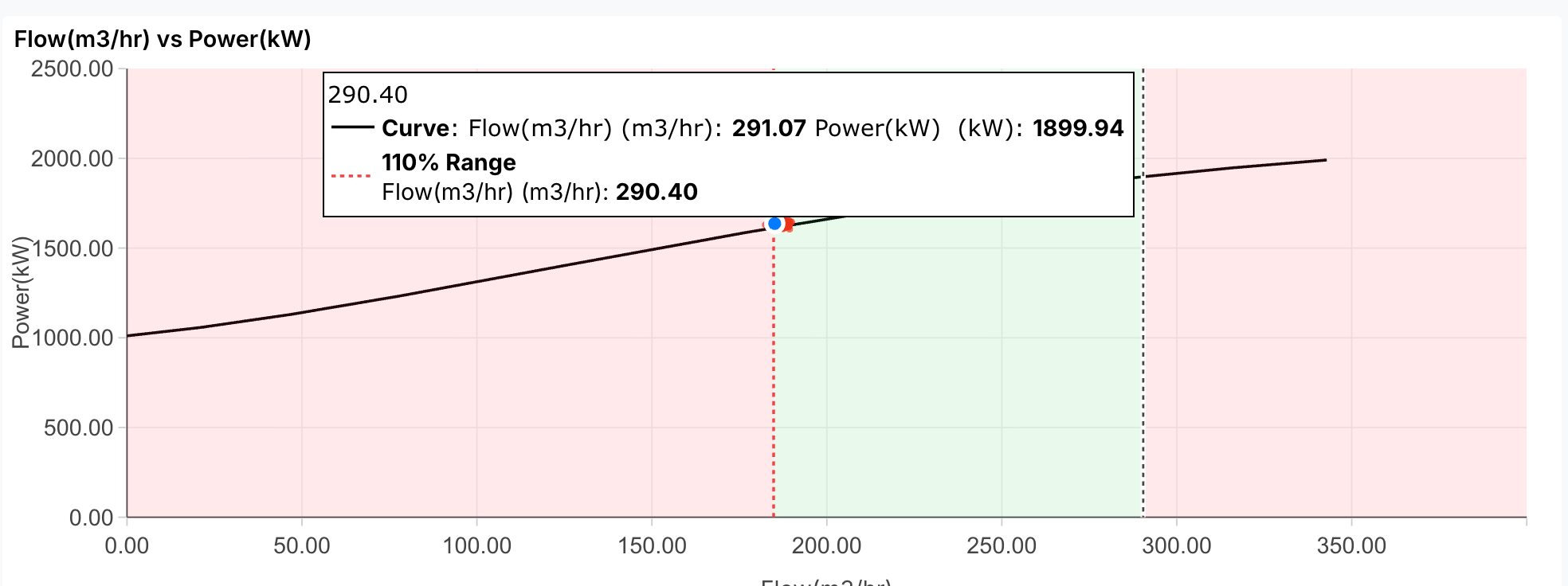
Figure 9. 110% = 290.40 m³/hr
The middle region (highlighted in green) represents the optimal operating range, where the equipment is expected to perform efficiently. The regions outside this range (highlighted in red) indicate deviation from the preferred operating conditions.
While these regions are not explicitly labeled as “safe” or “unsafe,” they are typically interpreted as:
- Green → Preferred operating range
- Red → Potential deviation or concern
The green zone essentially represents the valid operating range, derived directly from the BEP value.
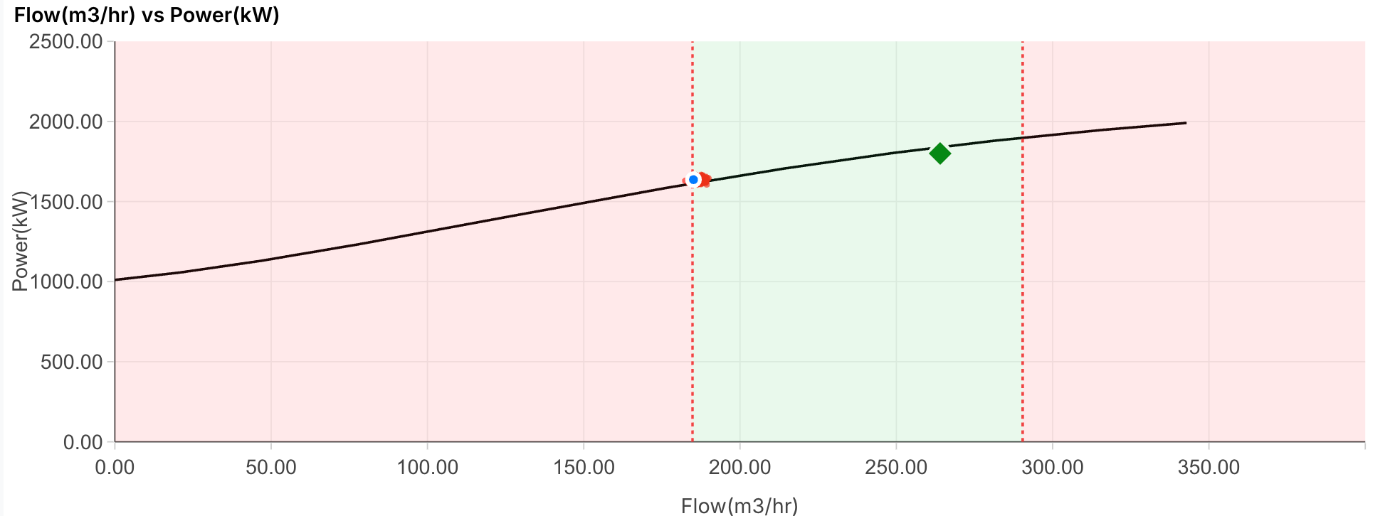
Figure 10. The green zone essentially represents the valid operating range,…
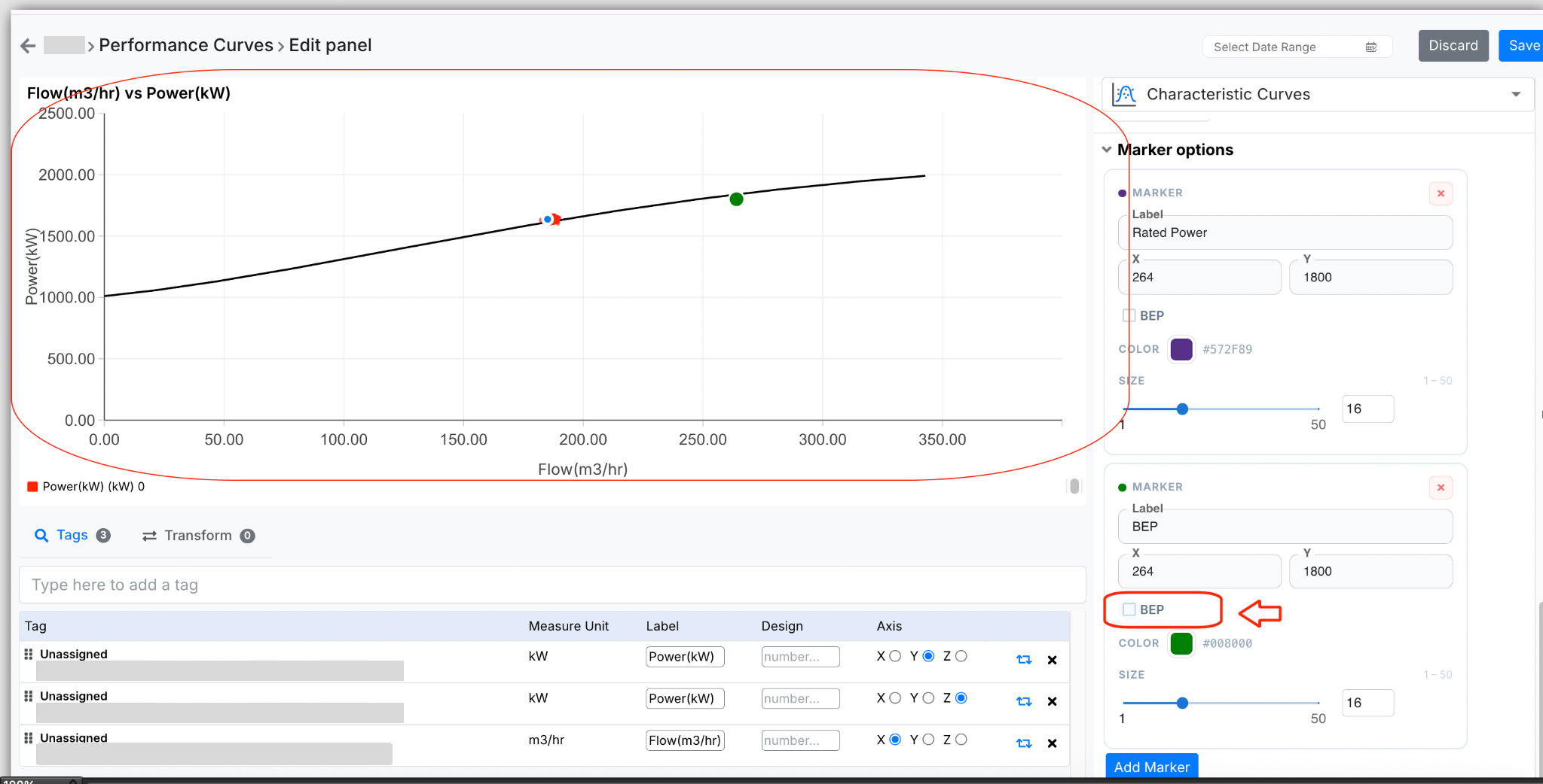
Figure 11. These color-coded zones are directly dependent on the BEP…
In addition to static markers, the graph also displays a dynamic marker:
- This represents the current operating condition
- It is plotted using real-time values
- If the system is not actively running, the last available value is shown
This allows users to instantly see how the system is performing relative to the design curve.
¶ Flexibility of Marker Configuration
The system allows adding multiple markers based on client requirements. While currently used for:
- BEP
- Rated point
It can also be extended to:
- Custom thresholds
- Inspection points
- Operational limits
¶ Interpreting the Curve
The characteristic curve is not just a visualization—it is a decision-support tool.
If the real-time values:
- Align closely with the curve → Equipment is operating as expected
- Fall below or above the curve → Indicates deviation
¶ Supporting Configurations
While the curve and markers form the core of the feature, additional configurations enhance usability:
- Tags section allows mapping and modifying input parameters
- Transform option (currently not in active use) can support aggregations
- Tooltip settings control how values are displayed on hover
- Font and legend settings improve readability
These are primarily presentation-level controls and do not affect the core logic of the curve.
¶ Overall Workflow
To summarize the complete flow:
- The client provides a performance curve →
- The curve is digitized and converted into mathematical form →
- A smooth design curve is generated →
- Real-time data is mapped onto this curve →
- Markers and operating zones are applied →
- The system continuously compares expected vs actual performance
¶ 10. Alert Generation and Monitoring Logic
The characteristic curve in the dashboard is not only used for visualization but also serves as the basis for performance monitoring and alert generation. The system continuously evaluates real-time operating data against the design curve to identify any deviation in performance.
¶ 10.1 Basis of Alert Calculation
Alert generation is based on a comparison between:
- Actual efficiency (real-time value)
- Design efficiency (value derived from the curve at the same flow)
For every operating point, the system performs a flow-specific evaluation. It identifies the expected efficiency from the curve corresponding to that flow and calculates a threshold value.
The threshold is defined as:
- 90% of the corresponding design efficiency value
An alert is triggered when:
- The actual efficiency goes beyond the acceptable threshold, i.e., it is beyond 90% of the design efficiency at that specific flow
This comparison is purely numerical and is not based on the visual position of the point on the graph.
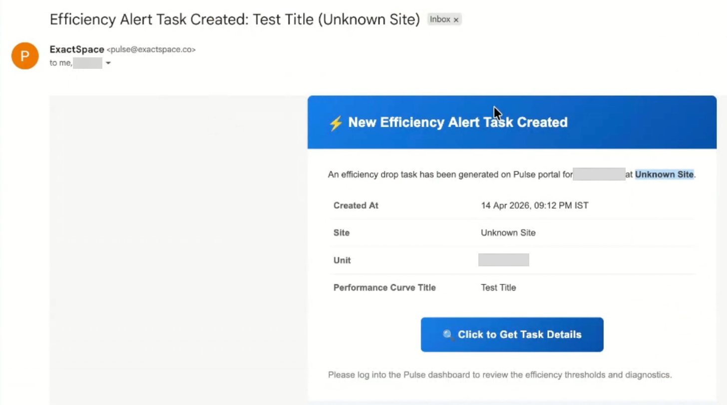
Figure 12. Basis of Alert Calculation
Referring to the characteristic curve shown. At a specific operating point:
- Flow (Capacity) = 296.83 m³/hr
- Design Efficiency (from curve) = 70.56%
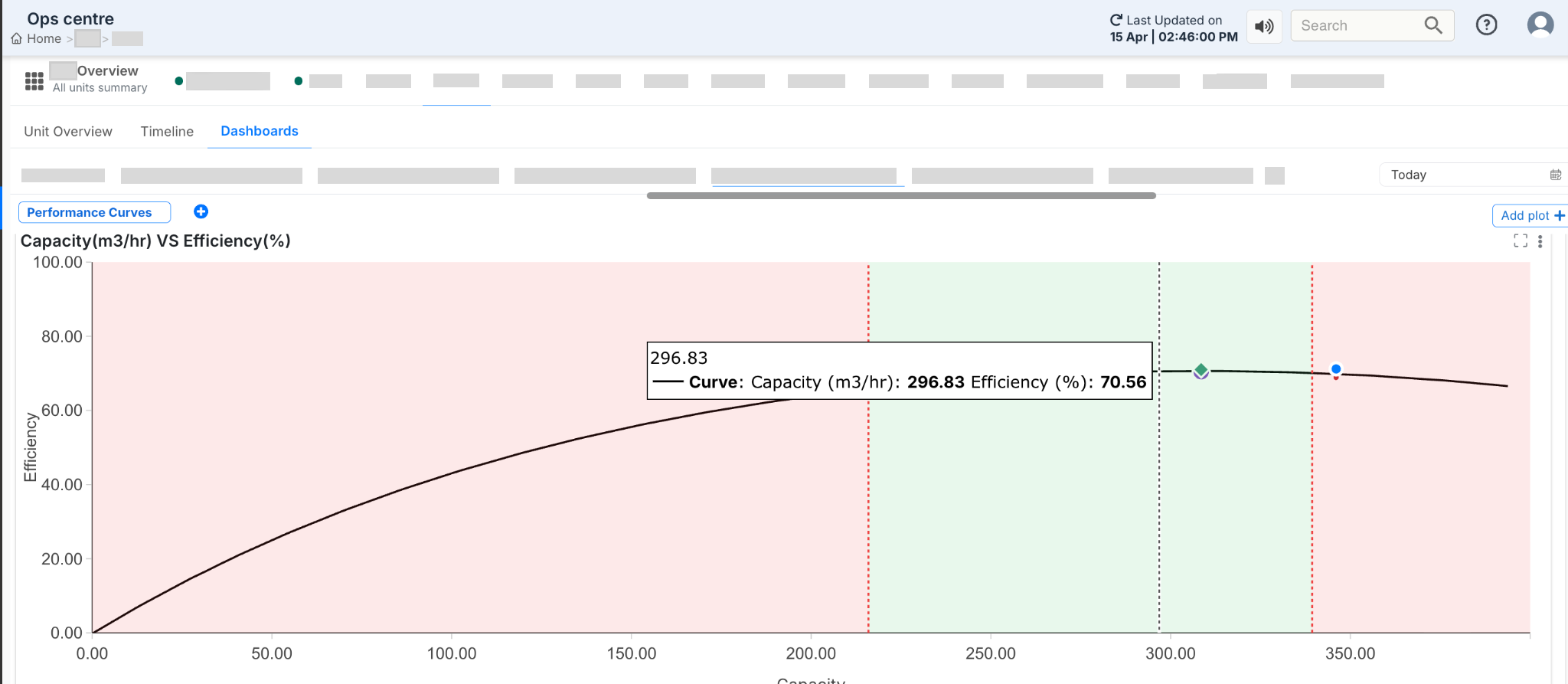
Figure 13. Example Based on Current Graph (Capacity vs Efficiency)
Step 1: Threshold Calculation: The alert threshold is calculated as:
Threshold= 90% × 70.56 = 63.50 %
Step 2: Comparison with Actual Value: The system compares this threshold with the actual efficiency plotted on the graph:
- If actual efficiency ≥ 63.50%
→ The system is operating within acceptable limits - If actual efficiency < 63.50%
→ The system has crossed the acceptable threshold → Alert is triggered
Step 3: Interpretation of Current Graph: In the current graph:
- The plotted operating point lies very close to the design curve
- This indicates that the actual efficiency is close to 70.56%
Since this value is significantly higher than the threshold (63.50%): The system is operating normally.No alert is generated
¶ 10.3 Clarification: BEP Zones vs Alert Logic
It is important to distinguish between the visual zones on the graph and the actual alert logic.
BEP-Based Zones (Green and Red Regions)
- Derived from 70% to 110% of BEP flow
- Represent the preferred operating range
- Help in visual interpretation of performance
Alert Logic
- Based on 90% of design efficiency
- Evaluated at each flow point
- Independent of BEP zones
Even if a point lies within the green zone, an alert can still be triggered if the efficiency falls beyond the acceptable threshold. Similarly, a point outside the green zone does not necessarily trigger an alert unless the efficiency condition is violated.
¶ 10.4 Notification and Task Workflow
When an alert condition is detected, the system initiates an automated workflow to track and manage the deviation.
- A task is generated to monitor the issue
- The task remains active for a 24-hour window
- An email notification is sent when the alert is first triggered
If the system recovers and efficiency returns to normal:
- A comment is added automatically indicating recovery
- The task is marked as completed
If the efficiency drops again after the 24-hour period:
- A new task is created
- A new notification cycle begins
¶ 10.5 Notification Control and Frequency
- To ensure effective communication without excessive alerts:
- Only one email notification is sent within a 24-hour period
- Subsequent updates are tracked through comments within the task
- No repeated emails are sent for every fluctuation
- This approach helps in:
- Avoiding notification overload
- Maintaining clear tracking of issues
- Ensuring meaningful alerts
¶ 10.6 Data Validation Consideration
- For accurate alert generation, it is important that:
- Real-time data points lie on or near the design curve
- Any significant deviation due to incorrect data is validated
- Incorrect data points may result in:
- False alerts
- Misinterpretation of system performance
Therefore, validation of plotted data is essential before relying on alert outputs.