¶ 1. Introduction
This document describes the Dashboard and Ops Centre module of the Pulse application. Pulse is a condition-monitoring and reliability platform that consolidates equipment health, incidents, and maintenance tasks for an industrial site into a single, role-based web application.
This manual is intended for engineers, operators, and reliability personnel who use Pulse to monitor the health of plant units, investigate incidents, track maintenance tasks, and build engineering dashboards. It is written so that a new user can understand, page by page, how the Dashboard module behaves and why particular colours, numbers, and navigation links appear where they do.
The screens referenced in this manual are illustrative. Site names, unit names, and numeric values shown in the figures are examples only and will vary from client to client and from moment to moment, as the data refreshes continuously from the connected plant systems. The navigation flow, terminology, colour codes, and underlying logic described here, however, remain the same across every Pulse deployment.
¶ 1.1 Scope
This manual covers the following areas of the Dashboard module:
-
Login and secure access to Pulse
-
The Dashboard (Ops Centre) landing page, including Asset Health, Uptime, and the Site Listing
-
The logic used to sort and colour-code assets and units on the Dashboard
-
Drilling down into Assets, Tasks, and Incidents from the Dashboard
-
The detailed Unit Overview page (KPI Status, Incidents, Task Summary, Asset Monitor)
-
Characteristic Performance Curves for rotating equipment
-
The Timeline tab, used for chronological incident analysis
-
The Dashboards tab, including creation of new dashboards, sections, and plots
-
A consolidated colour-code and glossary reference
¶ 2. Login
¶ 2.1 Purpose
The login process is the first step for users to access the Pulse application. It ensures secure, role-based access to site-specific data and functionality. Users must authenticate using their official credentials and a one-time password (OTP) generated by an authenticator app.
¶ 2.2 Accessing the Login Page
Login URL: https://<client-domain>.exactspace.co/pulse-login
The URL is specific to each client deployment and is provided to users by the site administrator during onboarding.
¶ 2.3 Login Steps
Follow the steps below to log in to the Pulse application:
-
Open Web Browser – Launch Chrome or Edge and enter the login URL in the address bar.
-
Enter Credentials – On the login page, enter the assigned username and password in the respective fields.
-
Click Login – After entering the registered credentials, click on the Login button.
-
Enter OTP from Authenticator App – The user receives a One-Time Password (OTP) in their registered authenticator app (e.g., Google Authenticator, Microsoft Authenticator). Enter the OTP into the designated field on the login screen. This is a multi-factor authentication (MFA) feature provided by Pulse for security purposes.
¶ 2.4 Successful Login and Redirection
Once authenticated, users are redirected to the Dashboard (Ops Centre) page, which is the main landing page of the application. The user should ensure the page loads completely without errors before proceeding.
¶ 2.5 Notes
-
Access to the application is restricted to authorised users only.
-
If a user forgets their password, they can reset it using the "Forgot Password" link on the Login page.
-
In case of login issues, contact the designated Pulse administrator for the site.
-
Ensure the system time on the user's device is synchronised, as an incorrect clock may impact OTP-based login.
¶ 3. Dashboard (Ops Centre) – Landing Page
The Dashboard, also referred to as the Ops Centre home page, is the primary monitoring page of Pulse. It provides a consolidated, real-time view of a client's operations by displaying overall equipment health, uptime, and a site-by-site summary of assets, tasks, and incidents on a single screen.
The information on the Dashboard refreshes periodically based on the latest data received from the connected plant systems, so that operators and engineers can identify abnormal operating conditions quickly and move directly to the relevant module for further analysis.
¶ 3.1 Layout Overview
When a user is connected to more than one unit or site, Pulse first opens an "All units summary" view. This view brings together three core panels side by side:
-
KPI Status – total KPIs monitored, and the count of Healthy versus Unhealthy KPIs, with a list of the KPIs currently outside their expected range.
-
Incidents – total active incidents, split by severity (Critical, Warning, Deviation), together with a trend graph and a list of the most recent incidents.
-
Task Summary – total tasks and their current status (Completed, In Progress, Not Started), together with a list of the most recently created or updated tasks.
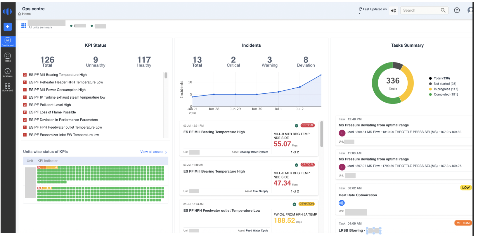
Figure 1. Ops Centre – All Units Summary view, showing KPI Status, Incidents, and Task Summary panels side by side
In the example above, the connected units report a combined KPI Status of 126 total KPIs, of which 117 are Healthy and 9 are Unhealthy; an Incidents panel showing 13 total incidents (2 Critical, 3 Warning, 8 Deviation) trending upward over the selected week; and a Task Summary of 336 tasks, of which 191 are Completed, 117 are In Progress, and 28 are Not Started.
¶ 3.2 Asset Health Status
Below the summary panels (or, when a single site is selected, at the top of the page) Pulse displays the Asset Health donut. This donut shows the total number of assets monitored at the site and the proportion of assets in each health category:
-
Healthy (green) – the asset has no open incidents affecting it.
-
Review (yellow/orange) – the asset has a deviation or warning-level condition that should be reviewed.
-
At Risk (red) – the asset has one or more critical conditions and needs immediate attention.
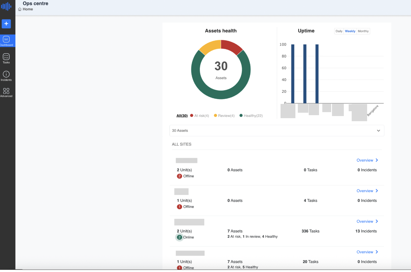
Figure 2. Asset Health donut and Uptime graph on the Dashboard landing page
In the example shown, the site has a total of 30 assets: 22 are Healthy (green), 4 are under Review (yellow), and 4 are At Risk (red). Clicking on any of the "All", "At risk", "Review", or "Healthy" labels below the donut filters the site list further down the page to show only the sites or units containing assets in that category.
¶ 3.3 Uptime Graph
Alongside the Asset Health donut, the Uptime graph provides a bar-chart view of the uptime percentage recorded across the connected sites. Users can toggle between Daily, Weekly, and Monthly views using the tabs above the graph to monitor performance over different time frames.
Each bar represents one connected site, and the height of the bar reflects the recorded uptime percentage for the selected period. This visual comparison allows a user to quickly identify any site whose uptime is lagging and may require attention.
¶ 3.4 Site / Unit Listing
Below the Asset Health and Uptime panels, Pulse lists every site or unit the logged-in user has access to. For each entry, the following information is displayed:
-
Number of Units Online – the count of process units under that site, together with an online/offline indicator. A green circle indicates the unit is currently online and reporting data; a red circle indicates the unit is offline (i.e., Pulse is not currently receiving live data from that unit, typically due to a communication or data-source interruption).
-
Number of Assets – the total assets configured for that site, broken down into At Risk, In Review, and Healthy counts, matching the same colour logic used in the Asset Health donut.
-
Number of Tasks – the total maintenance/operational tasks currently open or tracked for that site.
-
Number of Incidents – the total active incidents recorded for that site.
-
Overview – a link that opens the detailed Unit Overview page for that site (see Section 5).
In the reference screenshot, one site shows 2 Unit(s), both Online, with 7 Assets (2 At risk, 1 In review, 4 Healthy), 336 Tasks, and 13 Incidents; a neighbouring site shows 1 Unit, currently Offline, with 0 Assets and 4 Tasks recorded.
¶ 3.5 Navigating from the Site Listing
From the Dashboard landing page, users can navigate directly into the Assets, Tasks, or Incidents view for any site by clicking on the respective number displayed next to that site's name.
¶ 3.5.1 Viewing Unit-wise Status of KPIs (Assets Drill-down)
Clicking on the "No. of Assets" link for a site expands that section to display the Units-wise Status of KPIs table for the selected site.
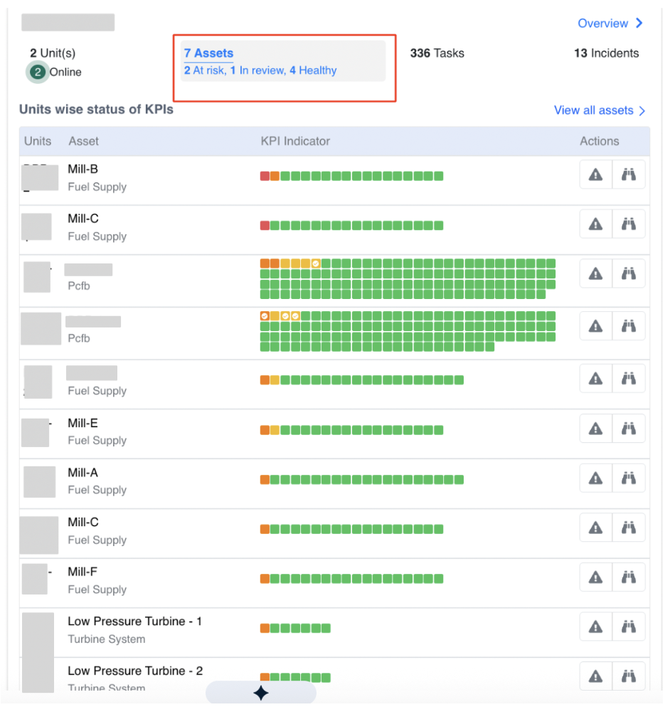
Figure 3. Units-wise Status of KPIs table, opened by clicking the Assets count for a site
This table lists every unit and asset under the selected site, together with a row of small coloured KPI-indicator blocks and two action icons on the right (a warning-triangle icon to raise or view alerts, and a binoculars icon to open the asset for detailed inspection).
¶ 3.5.2 Asset Matrix Display Logic (Sorting)
The Units-wise Status of KPIs table is not displayed in a random or alphabetical order. It follows a well-defined sorting logic based on the severity and distribution of incidents linked to each asset, so that the assets needing the most urgent attention are always shown at the top.
Each asset is represented using coloured fault-tree indicators, where:
-
Red indicates a critical issue,
-
Orange indicates a warning,
-
Yellow indicates a deviation, and
-
Green means no current incident.
Assets with more severe (red/orange) or more widespread issues are automatically positioned higher in the list.
Sorting Criteria
1. Incident Severity-Based Sorting
Each asset can have multiple fault trees, and each fault tree can have one active/open incident at a time. Each incident carries a severity level:
-
Critical (Red) = 3
-
Warning (Orange) = 2
-
Deviation (Yellow) = 1
-
No Incident (Green) = 0
The sorting prioritises assets with the highest severity incidents at the top: assets with critical (red) incidents come first, followed by those with warning (orange) incidents, then deviation (yellow) incidents, and finally assets with no open incidents (green only) are listed at the bottom.
Example: Consider two assets, Asset A and Asset B. Asset A has 3 fault trees, all showing critical-level issues (Red). Asset B has 4 fault trees, of which 3 are critical (Red) and 1 is slightly less severe (Orange). Even though both assets have critical issues, Asset B is placed above Asset A in the list, because Asset B has more fault trees affected — the issue is more widespread and may require quicker attention.
2. Number of Fault Trees with Incidents
If two or more assets share the same maximum severity level, the asset with more fault trees having open incidents appears higher in the list.
3. Green-Only Assets Sorting
For assets with no open incidents (all fault trees green), sorting falls back to the total number of fault trees configured — the asset with more fault trees appears higher.
This sorting logic helps operators and reliability engineers prioritise attention toward the most critical assets quickly and efficiently, without having to manually scan the entire list.
¶ 3.5.3 Task Summary Drill-down
Clicking on the "No. of Tasks" link for a site expands the section to display the Task Summary for that site, including a donut chart of task status and a list of individual tasks.
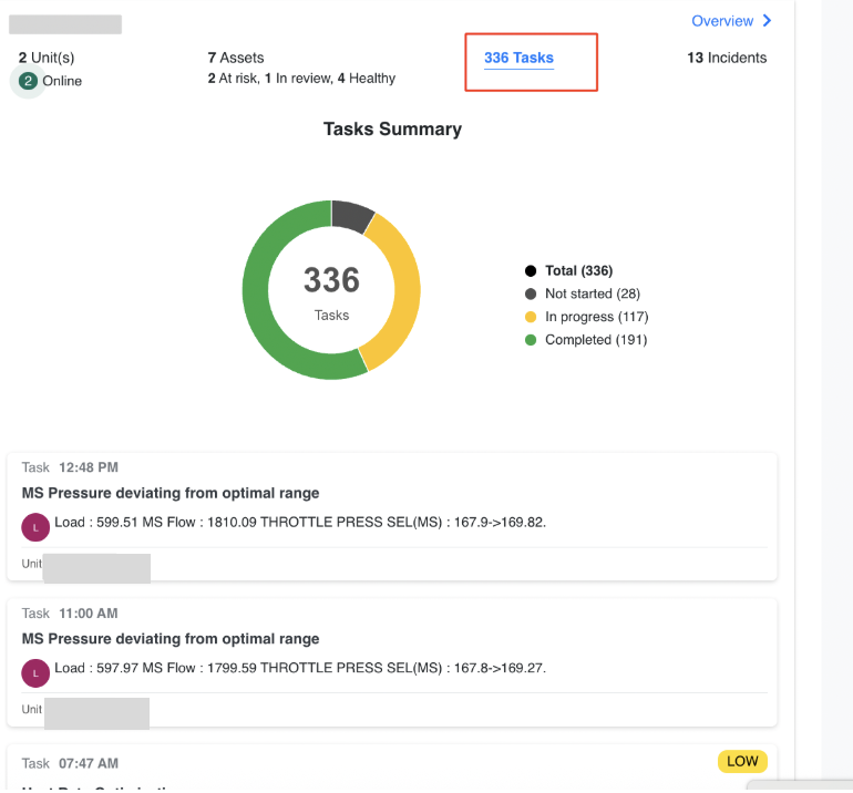
Figure 4. Task Summary drill-down, opened by clicking the Tasks count for a site
In the example shown, the site has 336 total tasks: 191 Completed (green), 117 In Progress (yellow), and 28 Not Started (grey). Below the donut, individual task cards list the task creation/update time, a short title describing the deviation or action, and key parameter values associated with that task.
¶ 3.5.4 Incident Summary Drill-down
Clicking on the "No. of Incidents" link for a site expands the section to display an incident trend graph and a summary list of incidents for that site.
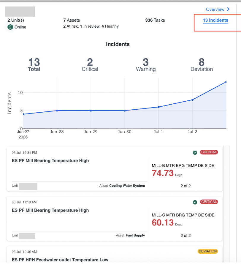
Figure 5. Incident Summary drill-down, opened by clicking the Incidents count for a site
The example above shows 13 Total incidents for the selected site, split into 2 Critical, 3 Warning, and 8 Deviation. The line graph plots the cumulative number of incidents recorded over the selected date range, allowing users to see at a glance whether incidents are trending upward or downward. Below the chart, individual incident cards display the date and time the incident was raised, the incident title, its severity tag (e.g., CRITICAL, DEVIATION), the affected tag/asset, and the current measured value.
Clicking on a specific incident card opens a pop-up window with detailed information about that incident, including a graphical representation of the relevant parameter values over time. From this pop-up, clicking "More Details" (bottom-right corner) redirects the user to the full Incidents page of Pulse, where a comprehensive view of the selected incident is available, including engineering comments, historical trends, and recommended actions.
¶ 3.6 Benefits Reported from the Incidents Page
The total savings realised through Pulse-assisted improvements can be viewed on the Incidents page. In the top-right corner, under the Actions tab, the Benefits Reported section displays the amount of benefit received. If benefits are received from multiple sources — either due to Pulse features directly or as a result of Pulse-assisted engineering improvements — the user can click the + button to add each entry. The system automatically calculates the total savings across all reported sources and displays the consolidated amount.
¶ 3.7 Opening the Detailed Unit Overview
Clicking the "Overview" link next to any site or unit on the Dashboard opens a new page providing detailed information about that unit — specific metrics, performance trends, historical data, and other key operational parameters. This detailed view is described fully in Section 5.
¶ 4. Ops Centre – Unit / Site Detail View
Selecting "Overview" for a unit from the Dashboard redirects the user to a detailed site-level view referred to as the Unit Overview. This page provides a comprehensive summary of the operational status, key performance indicators (KPIs), incident summary, and task assignments specific to that unit, enabling users to monitor the unit's health, identify problem areas, and take appropriate action based on real-time data.
¶ 4.1 Unit Navigation Bar
The top bar of the Unit Overview page displays a list of all units under the selected site. The currently selected unit is highlighted for easy reference, and the breadcrumb path above the bar shows the navigation path back to the Dashboard (for example, Fleet / <Unit Name>).
Users can switch between units (such as different process areas or equipment groups) by simply clicking the respective unit name in this bar, which reloads the page with the operational data and insights specific to that unit.
¶ 4.2 KPI Status Panel (Left)
The KPI Status panel summarises the health of all configured KPIs for the selected unit. It displays:
-
Total Fault Templates Deployed – the total number of fault-tree templates configured for the unit.
-
Healthy Fault Trees – shown in green, indicating KPIs currently within their expected operating range.
-
Unhealthy Fault Trees – shown in red, indicating KPIs currently outside their expected range and requiring attention.
Below the summary counts, Pulse lists the active (Critical / Warning / Deviation) alerts, each specifying the issue and the associated equipment. Critical alerts are prioritised at the top of the list and highlighted in red to indicate a high-priority concern; healthy or normal conditions are marked in green for quick visual distinction.
Colour Code: Red = Unhealthy KPI, Green = Healthy KPI.
¶ 4.3 Equipment-wise KPI Status
Located below the KPI list, this table offers a visual matrix of unit-level health. Each equipment item (for example, a mill, fan, turbine, or other rotating asset) is represented row-wise, and a grid of coloured boxes shows the condition of each KPI indicator configured for that equipment:
-
Green Box – the KPI is within acceptable limits.
-
Red / Orange / Yellow Box – the KPI has deviated from its acceptable range, with the exact shade indicating severity as described in Section 3.5.2 (Red = Critical, Orange = Warning, Yellow = Deviation).
This granular, colour-coded matrix helps users quickly identify which equipment items require inspection or action without opening each asset individually.
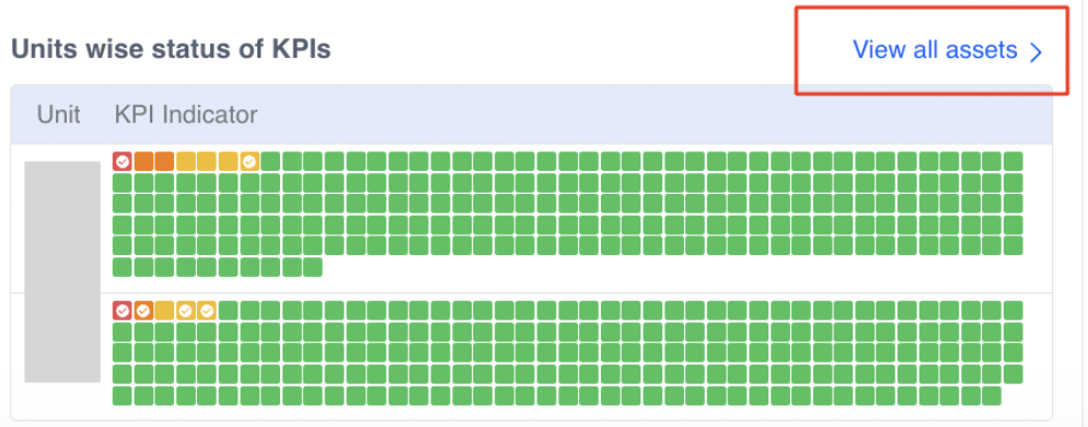
Figure 6. Units-wise Status of KPIs matrix with the "View all assets" link
Clicking the "View all assets" link redirects the user to the Asset Monitor page, described in Section 4.4.
¶ 4.4 Asset Monitor Page
The Asset Monitor page provides a centralised view of all monitored assets under the unit, along with their operational status, health indicators, and other key metrics.
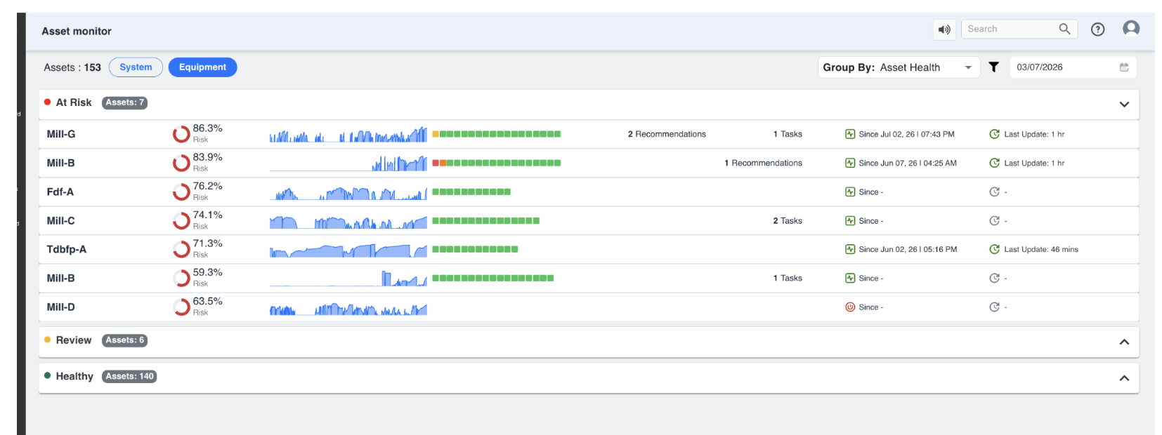
Figure 7. Asset Monitor page, grouped by Asset Health
Key elements of this page include:
-
Asset Count – the total number of assets under the current view (System or Equipment) is shown at the top-left, for example "Assets: 153".
-
View Toggle – users can switch between a System view (assets grouped by process system) and an Equipment view (assets grouped by equipment type) using the toggle buttons at the top.
-
Group By – assets can be grouped by Asset Health (At Risk, Review, Healthy) or by other available groupings, using the drop-down at the top-right.
-
Risk Gauge – each asset row shows a circular gauge with a percentage risk score; a higher percentage indicates a greater likelihood of near-term failure or performance deviation.
-
Trend Sparkline – a compact trend chart shows recent historical behaviour of the asset's key parameter.
-
KPI Indicator Row – the same coloured-box matrix described in Section 4.3, scoped to that specific asset's fault trees.
-
Recommendations / Tasks – the count of open recommendations and tasks linked to that asset, where applicable.
-
Since / Last Update – "Since" shows the date and time the asset entered its current risk state; "Last Update" shows how recently the asset's data was refreshed.
In the example shown, the At Risk group contains 7 assets with risk scores ranging from roughly 59% to 86%, the Review group contains 6 assets, and the Healthy group contains 140 assets. Each group can be expanded or collapsed using the arrow on the right of its header row.
¶ 4.4 Incidents Chart (Centre)
This chart shows the trend of incidents reported within the selected unit over a defined period. In the reference example (04 to 10 of a given month), the unit recorded a Total of 10 Incidents, of which 5 were Critical, 2 were Warnings, and 3 were Deviations.
The line chart visually depicts the change in incident count over time — in the example, critical incidents rise steadily toward the end of the selected period. Below the graph, a card view lists individual incident logs, along with timestamps and severity tags (for example, a CRITICAL tag shown in red), such as a pump gearbox bearing vibration reading recorded at 09:16 am.
¶ 4.5 Task Summary (Right)
A donut chart on the right-hand side of the Unit Overview page provides a snapshot of current task progress for the selected unit, broken down as Completed (green segment), In Progress (yellow segment), and Not Started (grey segment).
This section offers a quick status update on how many tasks are active, completed, or pending action for the unit.
¶ 4.6 Task List
Below the donut chart, in the rightmost task section, individual tasks are listed with the following information:
-
Task Time – the timestamp when the task was created or last updated.
-
Title – the name or short description of the task, typically describing the deviation or action required.
-
Priority Tag – a coloured tag (for example, LOW or MEDIUM) indicating the urgency of the task.
-
Assignee / Related Parameters – the user responsible for the task, or the key parameter values associated with it.
Clicking on any task redirects the user to the corresponding Task Details page, where they can view full information and perform actions related to that specific task, such as adding comments, updating status, or closing the task once resolved.
¶ 5. Characteristic Performance Curves
The Characteristic Curve is a visualisation feature available within the Dashboard section of Pulse, designed to provide a clear comparison between the design performance and the actual operating performance of industrial equipment such as pumps and compressors.
At its core, this feature transforms the static performance curves provided by the client into a dynamic, real-time analytical tool. It enables users to visually assess whether the equipment is operating within its expected performance range and identify any deviations that may indicate inefficiencies or potential issues.
¶ 5.1 Conceptual Understanding of the Characteristic Curve
The starting point is typically a datasheet performance graph supplied by the client, which represents how the equipment is expected to behave under different operating conditions. For example, in a typical pump datasheet:
-
The X-axis represents Capacity (Flow in m3/hr)
-
The Y-axis represents parameters such as Efficiency, Head, or Power
These curves define the intended design behaviour of the equipment. For instance, efficiency typically increases with flow up to a certain point (the Best Efficiency Point), and then starts decreasing. In Pulse, this concept is translated into a simple idea: "what should happen" (the design curve) is continuously compared with "what is happening" (real-time data).
¶ 5.2 How the Curve is Created in Pulse
Creating the characteristic curve is not a manual plotting exercise but a structured transformation process. Initially, the graph provided by the client is digitised: multiple points along the curve are identified, and their corresponding X (Flow) and Y (Efficiency / Head / Power) values are extracted.
These extracted points are then used to generate a mathematical representation of the curve. Instead of plotting discrete points, Pulse fits a smooth curve using regression, of the general form:
y = a0 + a1x + a2x2 + a3x3
where y is the intercept plus successive coefficients multiplying x, x2, and x3. This equation allows the system to recreate the curve accurately, generate values for any intermediate point, and maintain smoothness and continuity.
¶ 5.2.1 Curve Accuracy and Polynomial Degree
The accuracy of the generated curve depends on the degree of the polynomial used. A lower-degree polynomial (for example, linear) results in a simpler curve, whereas higher-degree polynomials allow the system to match more complex shapes from the client's datasheet. A simpler curve may use fewer coefficients, while a more complex curve requires higher-degree terms. The degree is selected iteratively to ensure the generated curve closely resembles the original client-provided performance curve, giving both visual accuracy and mathematical consistency.
¶ 5.2.2 Tag Value Range Constraint
When configuring the characteristic curve, it is important to ensure that the selected tags produce values within the defined X-axis range. For example, if the X-axis (Flow) range is defined from 0 to approximately 390, any tag mapped to the graph must produce values within this range. If tag values fall outside this range, the data points may not be plotted correctly and the curve visualisation may not behave as expected. It is therefore essential, while assigning tags, to ensure that the selected data aligns with the configured axis limits.
¶ 5.2.3 Mandatory Tag Configuration Requirement
The system requires a minimum number of tags to successfully create and save a characteristic curve:
-
At least three tags must be configured.
-
Each tag must be assigned to an axis (X, Y, or Z).
-
Even where the Z-axis is not functionally required (such as for pump-based curves), a third tag is still needed to satisfy the system's configuration requirement.
This ensures consistency in how characteristic curves are structured within the platform. The coefficients (intercept, x, x2, x3, and so on) are tuned until the generated curve closely matches the original client graph, which is why multiple coefficients appear in the configuration panel — they define the final shape of the curve.
¶ 5.3 Axis Configuration and Their Meaning
The axis configuration depends on the type of equipment being monitored. For pumps, the system works with a straightforward two-axis configuration: the X-axis represents Flow (m3/hr) and the Y-axis represents the parameter being tracked (Efficiency, Head, or Power). Since pump performance does not vary across multiple operating layers like speed curves, a third axis is not required.
In contrast, compressors often need an additional dimension. In such cases, the Z-axis represents operating conditions such as speed (RPM), and multiple curves may exist for different speeds. This allows the system to represent more complex performance behaviour, where the same flow may result in different outputs depending on operating conditions.
¶ 5.4 Real-Time Data Mapping
Once the curve is established, real-time data is mapped onto it. Each axis is linked to specific tags — Flow is typically a raw sensor value converted into standard units (m3/hr), while Efficiency, Head, or Power are either measured or calculated values. As data flows into the system, it is plotted dynamically on the graph, creating a continuous comparison between the design curve (black line) and the actual operating point (blue marker).
When a user hovers over the graph, detailed values are displayed, including actual versus design values, the timestamp, and marker information (such as BEP or the Rated point).
¶ 5.5 Understanding Markers
Markers are one of the most important additions to the characteristic curve feature, as they provide clear reference points defined by the client. These are not system-generated assumptions — they are based on actual datasheet values.
¶ 5.5.1 Types of Markers
-
Rated Point – represents the standard operating condition of the equipment.
-
Best Efficiency Point (BEP) – represents the point at which the equipment operates at maximum efficiency.
In many cases, both values are the same unless explicitly specified otherwise in the datasheet. The BEP and Rated values are derived from the equipment datasheet and represent design parameters — they are not dynamically calculated and remain constant unless manually updated. Any change would require manual reconfiguration in the system.
Each marker is defined using an X value (Flow), a Y value (Efficiency / parameter), and a label, colour, and size. Markers appear visually on the graph (for example, as a coloured diamond for BEP), making them easy to identify. The colour used for a marker is chosen purely for visual distinction and readability — it is not fixed or predefined, and there is no logic tied to a specific colour.
¶ 5.5.2 BEP-Based Operating Range
One of the key requirements is visualising the acceptable operating range around the BEP. This is implemented by calculating a range based on the BEP flow value: 70% of BEP flow and 110% of BEP flow. For example, if the BEP Flow is 239 m3/hr, then 70% equals 184.02 m3/hr and 110% equals 290.40 m3/hr.
Based on this calculation, the graph is visually divided into three regions. The middle region (highlighted in green) represents the optimal operating range, where the equipment is expected to perform efficiently. The regions outside this range (highlighted in red) indicate deviation from the preferred operating conditions. While these regions are not explicitly labelled "safe" or "unsafe", they are typically interpreted as green = preferred operating range and red = potential deviation or concern.
These colour-coded zones are directly dependent on the BEP configuration. If the BEP option is deselected from the marker settings, the system no longer displays the red and green background regions, and the graph reverts to showing only the characteristic curve without any shaded operating zones.
¶ 5.5.3 Current Operating Point
In addition to the static markers, the graph also displays a dynamic marker representing the current operating condition, plotted using real-time values. If the system is not actively running, the last available value is shown. This allows users to instantly see how the equipment is performing relative to the design curve.
¶ 5.5.4 Flexibility of Marker Configuration
The system allows adding multiple markers based on client requirements. While currently used for BEP and the Rated point, marker configuration can also be extended to custom thresholds, inspection points, or other operational limits.
¶ 5.6 Interpreting the Curve
The characteristic curve is a decision-support tool, not just a visualisation. If real-time values align closely with the curve, the equipment is operating as expected; if values fall below or above the curve, this indicates a deviation from design performance.
¶ 5.7 Supporting Configurations
While the curve and markers form the core of the feature, additional configurations enhance usability:
-
Tags section allows mapping and modifying input parameters.
-
Transform option (currently not in active use) can support aggregations.
-
Tooltip settings control how values are displayed on hover.
-
Font and legend settings improve readability.
These are primarily presentation-level controls and do not affect the core logic of the curve.
¶ 5.8 Overall Workflow
To summarise the complete flow: the client provides a performance curve, the curve is digitised and converted into mathematical form, a smooth design curve is generated, real-time data is mapped onto this curve, markers and operating zones are applied, and the system continuously compares expected versus actual performance.
¶ 5.9 Alert Generation and Monitoring Logic
The characteristic curve is not only used for visualisation but also serves as the basis for performance monitoring and alert generation. The system continuously evaluates real-time operating data against the design curve to identify any deviation in performance.
¶ 5.9.1 Basis of Alert Calculation
Alert generation compares the actual efficiency (real-time value) with the design efficiency (the value derived from the curve at the same flow). For every operating point, the system performs a flow-specific evaluation: it identifies the expected efficiency from the curve corresponding to that flow, and calculates a threshold value defined as 90% of the corresponding design efficiency value.
An alert is triggered when the actual efficiency falls beyond this threshold — that is, below 90% of the design efficiency at that specific flow. This comparison is purely numerical and is not based on the visual position of the point on the graph.
¶ 5.9.2 Worked Example
Consider an operating point where Flow (Capacity) = 296.83 m3/hr and Design Efficiency (from the curve) = 70.56%, representing the expected performance at that flow.
Step 1 — Threshold Calculation: Threshold = 90% x 70.56 = 63.50%.
Step 2 — Comparison with Actual Value: If actual efficiency is greater than or equal to 63.50%, the system is operating within acceptable limits. If actual efficiency is less than 63.50%, the system has crossed the acceptable threshold and an alert is triggered.
In this example, since the actual efficiency is close to the design value of 70.56% — well above the 63.50% threshold — the system is operating normally and no alert is generated.
¶ 5.9.3 Clarification: BEP Zones versus Alert Logic
It is important to distinguish between the visual zones on the graph and the actual alert logic:
-
BEP-Based Zones (green and red regions) are derived from 70% to 110% of BEP flow and represent the preferred operating range for visual interpretation.
-
Alert Logic is based on 90% of design efficiency, evaluated at each flow point, independently of the BEP zones.
Even if a point lies within the green zone, an alert can still be triggered if the efficiency falls beyond the acceptable threshold. Similarly, a point outside the green zone does not necessarily trigger an alert unless the efficiency condition is violated.
¶ 5.9.4 Notification and Task Workflow
When an alert condition is detected, the system initiates an automated workflow to track and manage the deviation:
-
A task is generated to monitor the issue.
-
The task remains active for a 24-hour window.
-
An email notification is sent when the alert is first triggered.
-
If the system recovers and efficiency returns to normal, a comment is added automatically indicating recovery, and the task is marked as completed.
-
If efficiency drops again after the 24-hour period, a new task is created and a new notification cycle begins.
¶ 5.9.5 Notification Control and Frequency
To ensure effective communication without excessive alerts, only one email notification is sent within a 24-hour period; subsequent updates are tracked through comments within the task, and no repeated emails are sent for every fluctuation. This approach avoids notification overload while maintaining clear tracking of issues and ensuring meaningful alerts.
¶ 5.9.6 Data Validation Consideration
For accurate alert generation, it is important that real-time data points lie on or near the design curve, and that any significant deviation due to incorrect data is validated. Incorrect data points may result in false alerts or misinterpretation of system performance; validating plotted data is therefore essential before relying on alert outputs.
¶ 6. Unit Overview, Timeline, and Dashboards Tabs
After selecting Overview for a unit from the Dashboard, the Ops Centre workspace opens for that unit. The selected unit remains active throughout the session, ensuring that all information displayed relates only to that unit. This workspace is organised into three tabs:
-
Unit Overview — the summary view described in Sections 4 and 5.
-
Timeline — a chronological view of incidents and deviations (Section 6.1).
-
Dashboards — configurable engineering dashboards (Section 6.2).
Each tab provides a different perspective of the same unit, allowing users to switch between summary information, event history, and engineering dashboards without leaving the workspace.
¶ 6.1 Timeline Tab
The Timeline tab provides a chronological view of incidents and deviations recorded within the selected unit. Instead of displaying events as a simple list, the Timeline presents them against a time scale, making it easier to understand when an event started, how long it remained active, and whether multiple events occurred simultaneously.
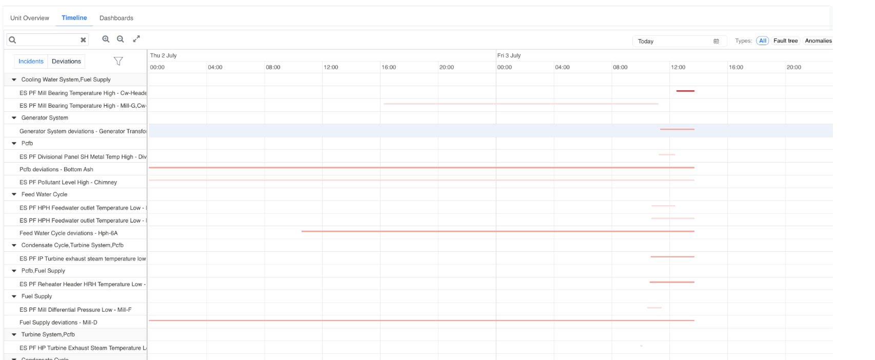
Figure 8. Timeline tab, showing equipment hierarchy on the left and event bars plotted against time on the right
Key elements of the Timeline tab:
-
Incidents / Deviations toggle — switches the left-hand list between active incidents and recorded deviations.
-
Equipment Hierarchy (left) — displays the process systems and equipment groups for the unit, together with the specific fault-tree event recorded against each (for example, a bearing-temperature-high event under a cooling-water or fuel-supply group).
-
Timeline Bars (right) — each row shows one or more horizontal bars representing the duration an event remained active. Darker/solid bars typically indicate longer-running or still-open events, while shorter bars represent brief or resolved events.
-
Date Selector — lets the user choose the day, or range of days, to display (for example, "Today").
-
Type Filters — All, Fault tree, and Anomalies filters let the user narrow the timeline to a specific event category.
-
Search, Zoom, and Expand controls — a search box lets users locate a specific equipment or event by name; zoom-in/zoom-out and expand-to-full-screen controls make it easier to inspect dense periods of activity.
The Timeline is particularly useful during troubleshooting, as it helps engineers determine whether multiple events occurred at the same time, or whether one event may have triggered another. By analysing the sequence of events, engineers can better understand the progression of an operational issue before performing detailed root-cause analysis.
¶ 6.2 Dashboards Tab
The Dashboards tab provides engineering dashboards configured for the selected unit. Unlike the Unit Overview page, which displays operational summaries, these dashboards provide detailed process visualisations and engineering KPIs, and can be created and customised by users with the appropriate permissions.
¶ 6.2.1 Dashboard and Section Structure
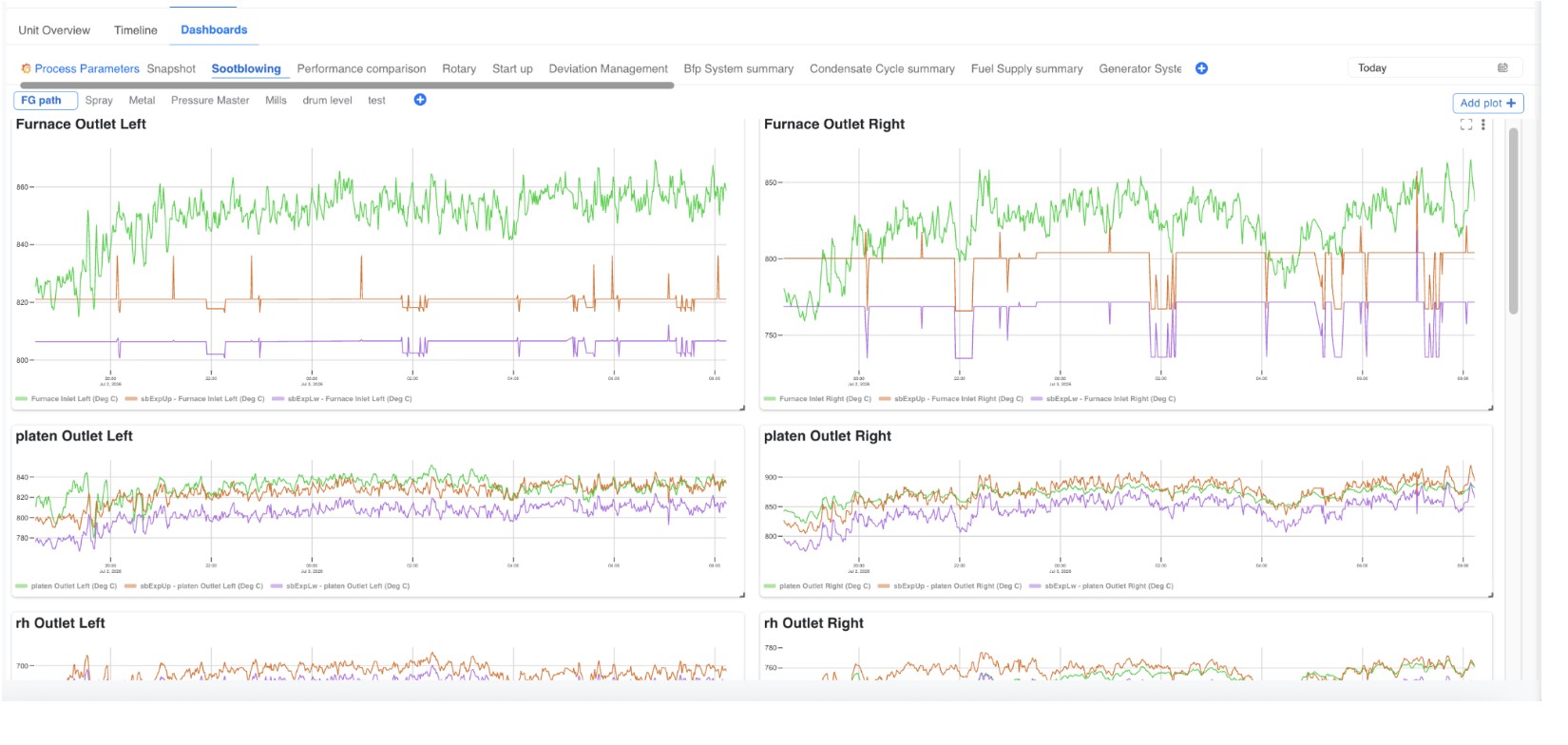
Figure 9. Dashboards tab, showing multiple dashboard tabs and section sub-tabs with line-plot panels
Each dashboard is organised into top-level tabs based on the configured process or equipment group. Depending on the project implementation, examples may include Process Parameters, Snapshot, Sootblowing, Performance Comparison, Rotary, Start-up, Deviation Management, or system-specific summaries (for example, a Feed-water/Condensate summary, Fuel Supply summary, or Generator System summary).
Within each top-level dashboard, content is further organised into sections (secondary tabs), for example FG Path, Spray, Metal, Pressure, or Mills, allowing related plots to be grouped together for a specific sub-system. Selecting a dashboard or section tab updates the page to display the corresponding set of plots.
A dashboard may include a mix of visualisation types, such as:
-
Line/trend plots comparing multiple tags over time (for example, an inlet temperature alongside its upper and lower expected limits).
-
Gauges showing a single live value against a configured minimum/maximum range.
-
XY plots, scatter plots, or contour plots for engineering analysis.
-
KPI indicator panels and other supported widgets.
In a typical trend plot, three coloured traces are commonly used together: the green trace represents the actual measured value, while the orange and purple traces represent the configured upper and lower expected limits for that parameter, making it easy to see at a glance when the actual value moves outside its expected band.
¶ 6.2.2 Creating a New Dashboard
Users with the appropriate permissions can create custom dashboards to organise process parameters and visualisations according to their own monitoring and reporting requirements.
To create a new dashboard:
-
Open the Dashboards tab from the Ops Centre workspace.
-
Click the + (Add) icon displayed at the end of the row of dashboard tabs.

Figure 10. The + (Add) icon used to create a new dashboard, located at the end of the dashboard tab row
This opens the Create New Dashboard window.
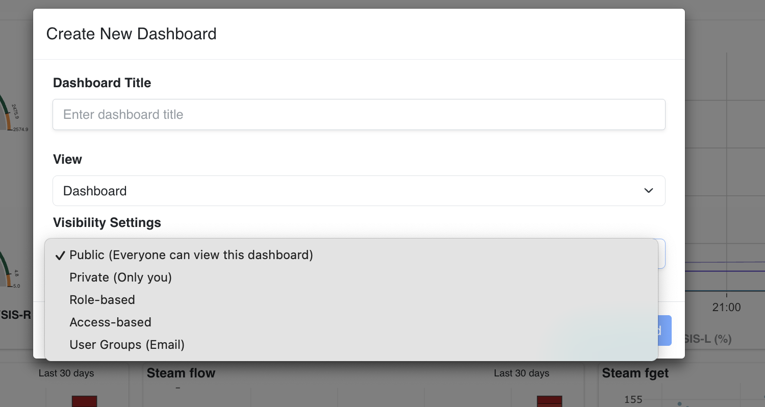
Figure 11. Create New Dashboard window, showing Dashboard Title, View, and Visibility Settings
In the Create New Dashboard window, enter the following information:
-
Dashboard Title — a meaningful name for the new dashboard.
-
View — the dashboard view type, selected from the available options (for example, a standard Dashboard view).
-
Visibility Settings — controls who can see and use the dashboard once created:
-
Public (Everyone can view this dashboard) — visible to all users who have access to the unit.
-
Private (Only you) — visible only to the user who created it.
-
Role-based — visible to users holding a specified role.
-
Access-based — visible according to a configured access/permission group.
-
User Groups (Email) — visible to a specific list of users identified by e-mail address.
-
After entering the required information, click Create Dashboard. The new dashboard is added to the list of available dashboard tabs and can be selected like any other dashboard.
¶ 6.2.3 Adding a Section to a Dashboard
Within a dashboard, related plots can be grouped into sections (the secondary row of tabs, such as Boiler, Turbine, or Mills). To add a new section, click the + icon next to the existing section tabs; this opens the Add Section window, where the user enters a Name for the section and clicks Save.
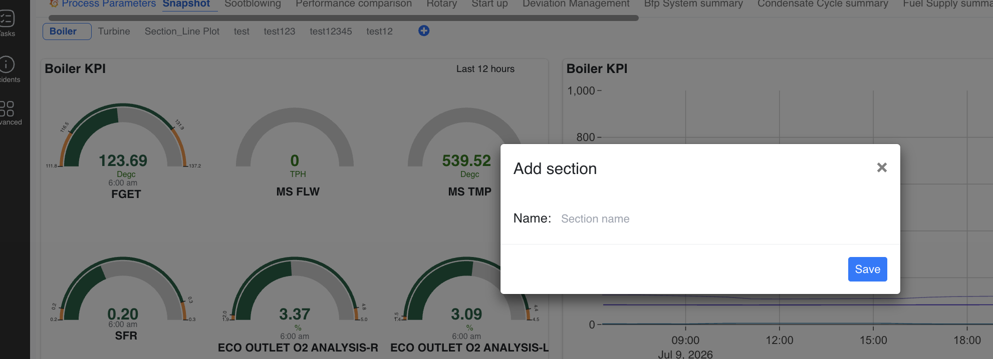
Figure 12. Add Section window, used to create a new grouping of plots within a dashboard; the Snapshot view shown here uses gauge widgets
The example above also illustrates a Snapshot-type dashboard, which favours gauge widgets over trend plots. Each gauge displays a single live reading (for example, a furnace exit gas temperature, steam flow, steam temperature, fuel-to-air ratio, or an oxygen-analysis reading) against its configured low/high band, with the current value and its measurement unit shown at the centre of the gauge, and the reading time noted below it. A matching line-plot version of the same parameter, showing the last 12 hours (or a similarly configured window), can be placed alongside the gauge for historical context.
¶ 6.2.4 Adding and Configuring a Plot
Within any section, clicking the Add Plot button at the top-right of the panel area opens a new, unconfigured plot panel and its associated Edit Panel view.
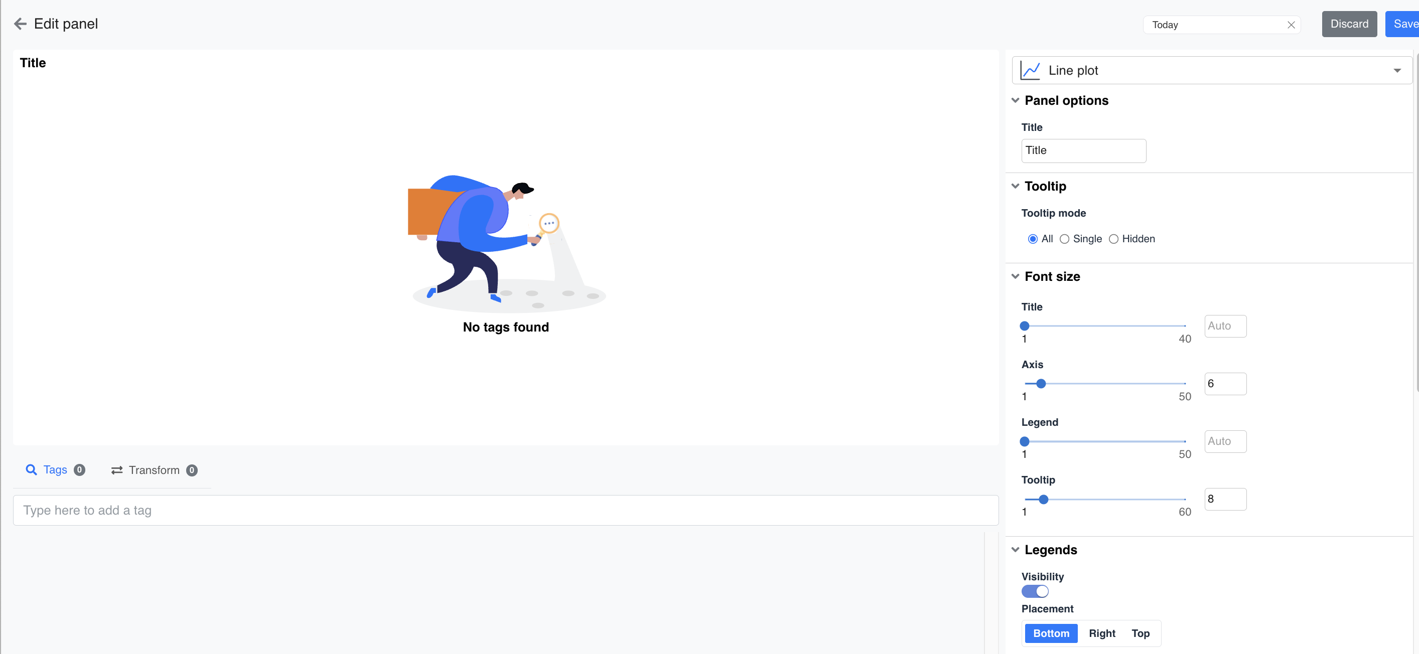
Figure 13. Edit Panel view for a newly added plot, showing plot type, panel options, tooltip, font size, and legend settings
The Edit Panel provides the following configuration options:
-
Plot Type — a drop-down at the top of the panel (for example, Line plot) lets the user choose the visualisation type for this panel.
-
Panel Options — Title, used to label the panel.
-
Tooltip — Tooltip mode controls how hover information is displayed: All (show every trace's value), Single (show only the nearest trace), or Hidden (no tooltip).
-
Font Size — independent sliders (each on a 1–40/1–50/1–60 scale, or set to Auto) control the size of the:
-
Title text
-
Axis labels
-
Legend text
-
Tooltip text
-
-
Legends — a Visibility toggle shows or hides the legend entirely, and a Placement control positions the legend at the Bottom, Right, or Top of the panel.
-
Tags — a search field used to add one or more process tags to the plot; until at least one tag is added, the panel displays a "No tags found" placeholder.
-
Transform — optional aggregation or calculation applied to the selected tag(s) before plotting.
Once the required tags and formatting options are configured, clicking Save (top-right of the Edit Panel) commits the plot to the dashboard section; clicking Discard exits without saving changes.
¶ 7. Colour Code and Status Reference
Because Pulse relies heavily on colour to communicate status at a glance, the table below consolidates every colour convention used across the Dashboard module in one place.
| Context | Colour | Meaning |
| Asset Health donut / Site listing | Green | Healthy — no open incidents affecting the asset |
| Yellow / Orange | Review — a deviation or warning-level condition exists that should be reviewed | |
| Red | At Risk — one or more critical conditions exist; immediate attention required | |
| Unit online/offline indicator | Green circle | Unit is online and actively reporting live data |
| Red circle | Unit is offline — Pulse is not currently receiving live data from the unit | |
| Fault-tree / KPI indicator blocks | Green | KPI/fault tree is within acceptable limits (no incident, severity 0) |
| Yellow | Deviation-level incident (severity 1) | |
| Orange | Warning-level incident (severity 2) | |
| Red | Critical-level incident (severity 3) — highest priority | |
| Task status donut | Grey | Not started |
| Yellow | In progress | |
| Green | Completed | |
| Characteristic curve BEP zone | Green band | Preferred operating range (70%–110% of BEP flow) |
| Red band | Deviation from preferred operating range | |
| Characteristic curve trace | Black line | Design curve, derived from the client datasheet |
| Blue marker | Actual real-time operating point |
Note: within a fault-tree or KPI indicator matrix, the overall sort order and the colour of an individual block always follow the severity ranking Critical (Red) > Warning (Orange) > Deviation (Yellow) > No Incident (Green), as described in Section 3.5.2.
¶ 8. Glossary
| Term | Definition |
| Asset | A piece of equipment or a logical grouping of equipment being monitored by Pulse (for example, a mill, pump, or turbine). |
| Fault Tree | A configured diagnostic model that evaluates one or more process conditions for a given asset and raises an incident when a defined condition is met. |
| KPI | Key Performance Indicator — a monitored parameter or fault-tree outcome used to judge the health of an asset or unit. |
| Incident | An operational abnormality or issue raised as an alarm by a fault tree, sensor threshold, or field observation, and tracked through to closure. |
| Task | A unit of work created (manually or automatically, for example from an incident or an alert) to investigate or resolve an issue, and tracked through to completion. |
| Severity | The priority level assigned to an incident: Critical, Warning, or Deviation, ranked in that order of urgency. |
| Uptime | The percentage of time a site or unit has been operating and reporting data over a selected period (Daily, Weekly, or Monthly). |
| BEP | Best Efficiency Point — the flow at which a pump or compressor operates at its maximum efficiency, as defined in the equipment datasheet. |
| Rated Point | The standard/design operating condition of the equipment, as defined in the equipment datasheet. |
| Characteristic Curve | A digitised, regression-fitted representation of an equipment's design performance curve, used to compare actual versus expected performance in real time. |
| Timeline | A chronological, time-scaled view of incidents and deviations for a unit, used to analyse the sequence and overlap of events. |
| Snapshot Dashboard | A dashboard type that favours gauge-style widgets showing current live readings, typically alongside a short-history trend plot. |